
JUWAN HA
Ph.D. in Design, North Carolina State University
jha4 [at] ncsu.edu
Research
Advanced HVAC Control
Advanced HVAC Control
Differentiable Predictive Control (DPC) for Multi-zone VAV System (2025 PNNL Summer Internship)
Overview
This study demonstrates physics-informed differentiable predictive control for supply-air-temperature reset in a reference office building with stochastic occupancy. A controller trained on a single HVAC zone was evaluated across five zones on the same floor and then deployed without retraining across all 15 zones in the building, balancing occupant comfort and HVAC energy use.
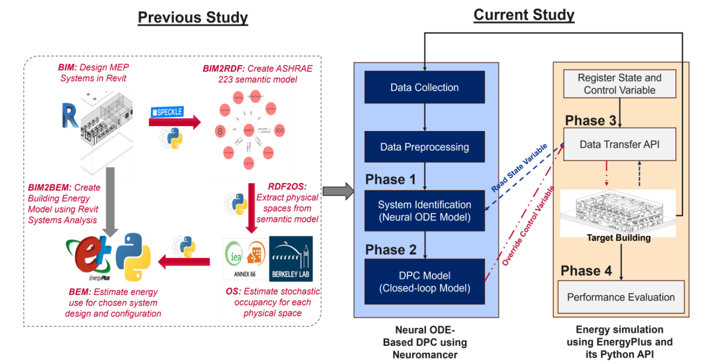
Neural ODE-Based Temperature Prediction
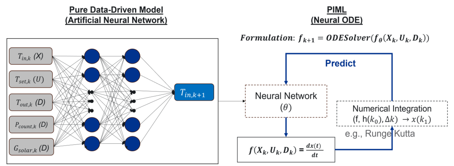
A Neural Ordinary Differential Equation (Neural ODE) model learns the rate of change in zone temperature from the current indoor temperature, supply-air setpoint, outdoor temperature, occupant count, and solar irradiance. Numerical integration using the fourth-order Runge–Kutta method produces a 24-hour temperature forecast, which serves as the predictor for differentiable predictive control. Trained on a single zone, the model achieved a test mean absolute error of 0.108 °C in that zone and was transferred to the remaining zones without retraining.
Key Results
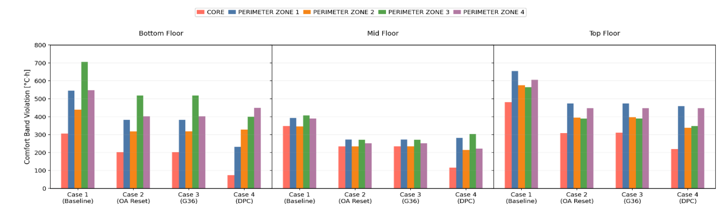
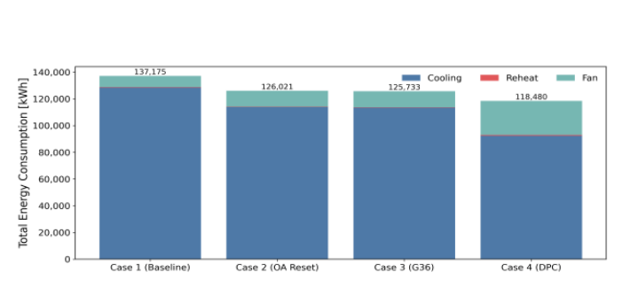
- Five-zone deployment during the representative cooling week: 54.8% fewer occupied comfort violations and 21.3% lower total HVAC energy use compared with rule-based control strategies.
- Whole-building zero-shot deployment across 15 zones during the cooling season: 39% fewer comfort violations and 14% lower total HVAC energy use.
Reference
A Whole-Building Demonstration of Differentiable Predictive Control with Stochastic Occupant Behavior
Juwan Ha, Ammar H.A. Dehwah, Karthikeya Devaprasad, and Michael Poplawski
SimBuild 2026 — 12th National Conference of IBPSA-USA, Minneapolis, Minnesota, May 20–22, 2026 (Best Paper in Controls).
Advanced HVAC Control
Differentiable Predictive Control (DPC) for Lighting System Control (2026 PNNL Summer Internship)
Overview
This ongoing research investigates occupancy-based lighting control, with the goal of reducing unnecessary lighting operation while maintaining lighting availability when spaces are occupied. The modeling and evaluation framework examines stochastic occupancy, passive infrared (PIR) motion-sensor signals, and the trade-off between false-on events (energy waste) and false-off events (lighting comfort violations).
Occupancy and Motion Sensor Modeling
Ground-truth occupant counts are generated by a stochastic occupancy simulator at five-minute intervals and converted to binary presence signals. PIR sensors are modeled using motion events associated with changes in occupant count, followed by a hold time. This distinguishes actual occupancy presence from the motion signal available to the controller.
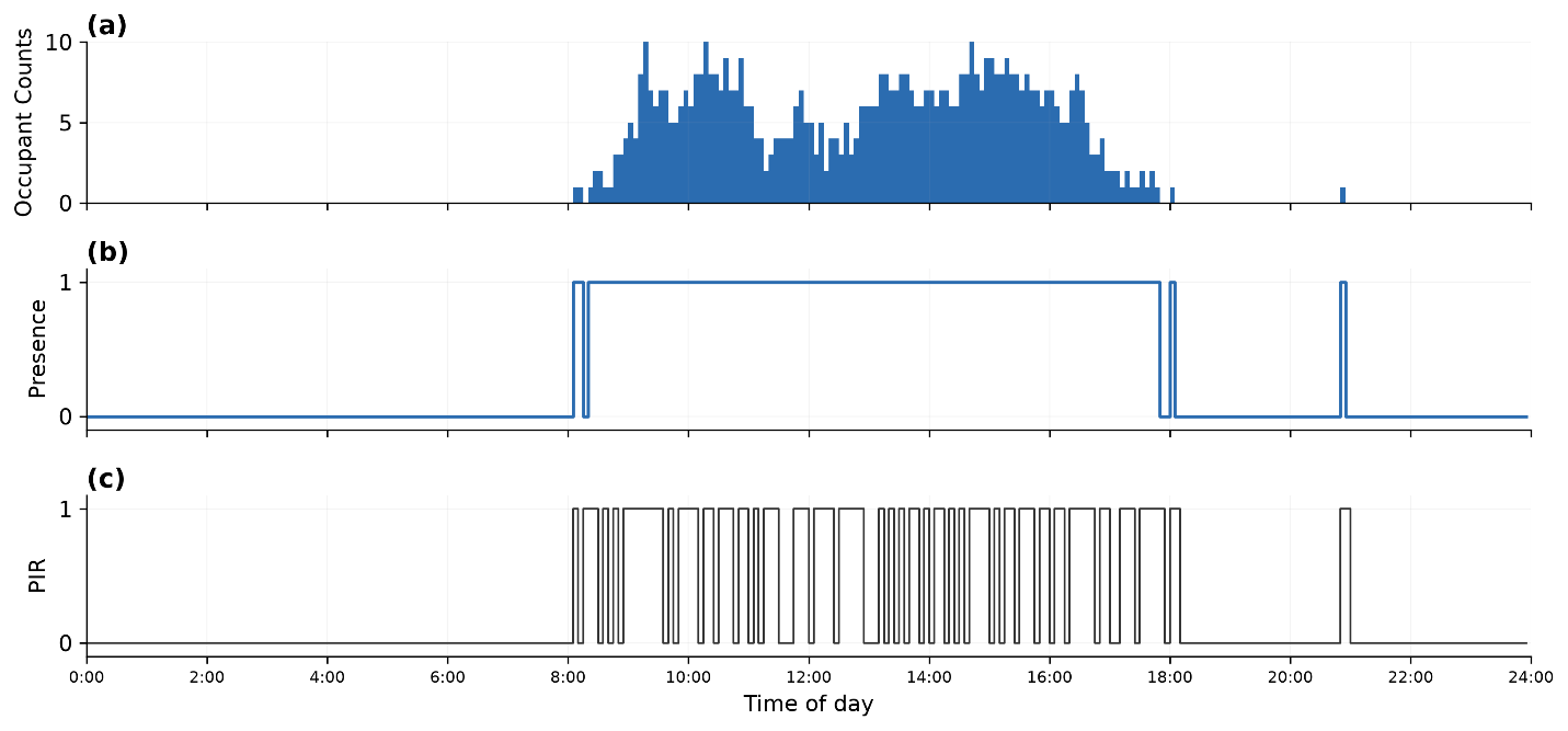
False-off Events
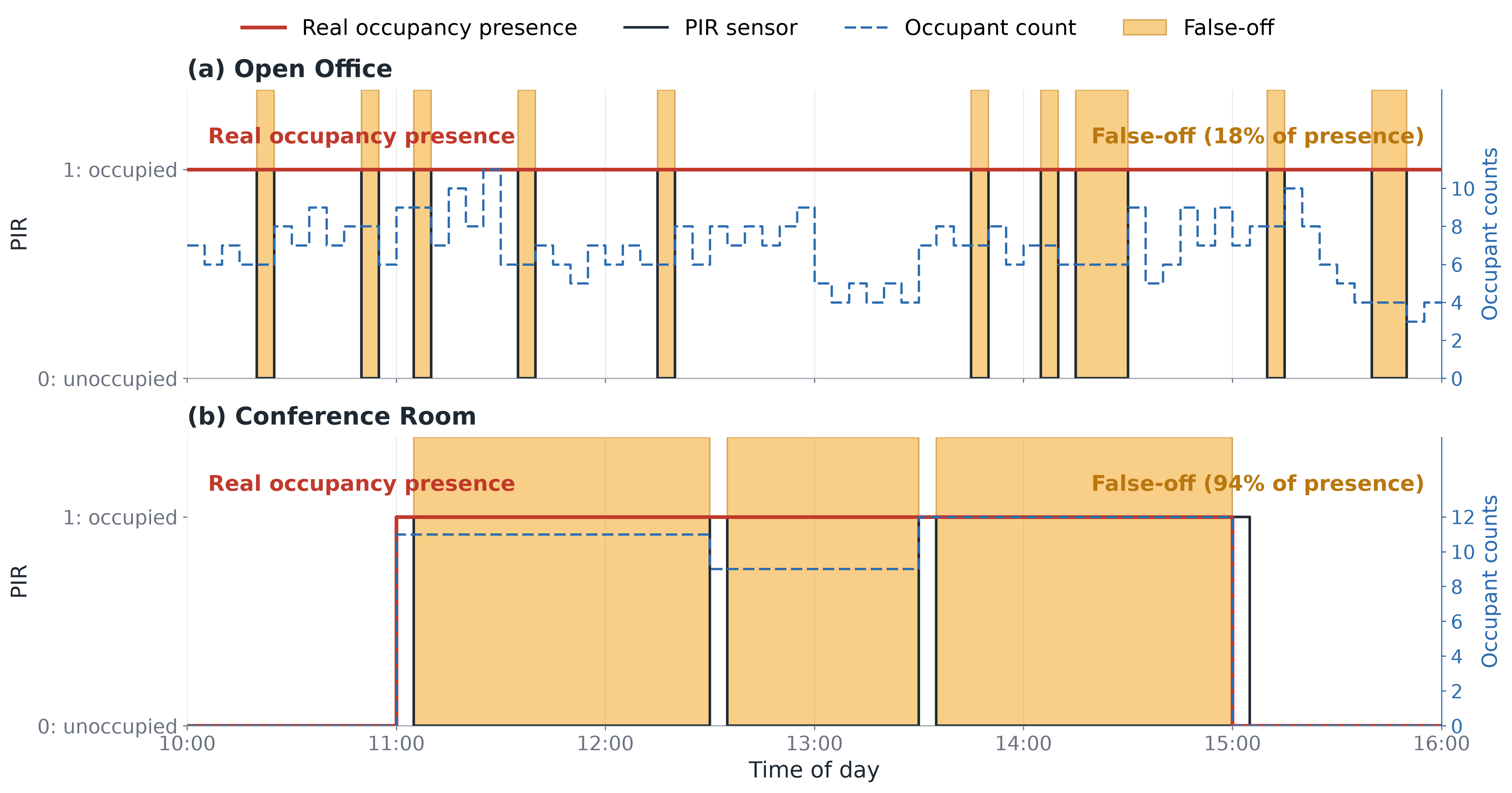
Motion sensors can indicate an unoccupied space even while people remain present. This occurs when occupants are relatively still, such as during seated office work or long meetings. The illustrated examples show false-off intervals in an open office and a conference room, highlighting the limitations of using motion detection alone for lighting control.
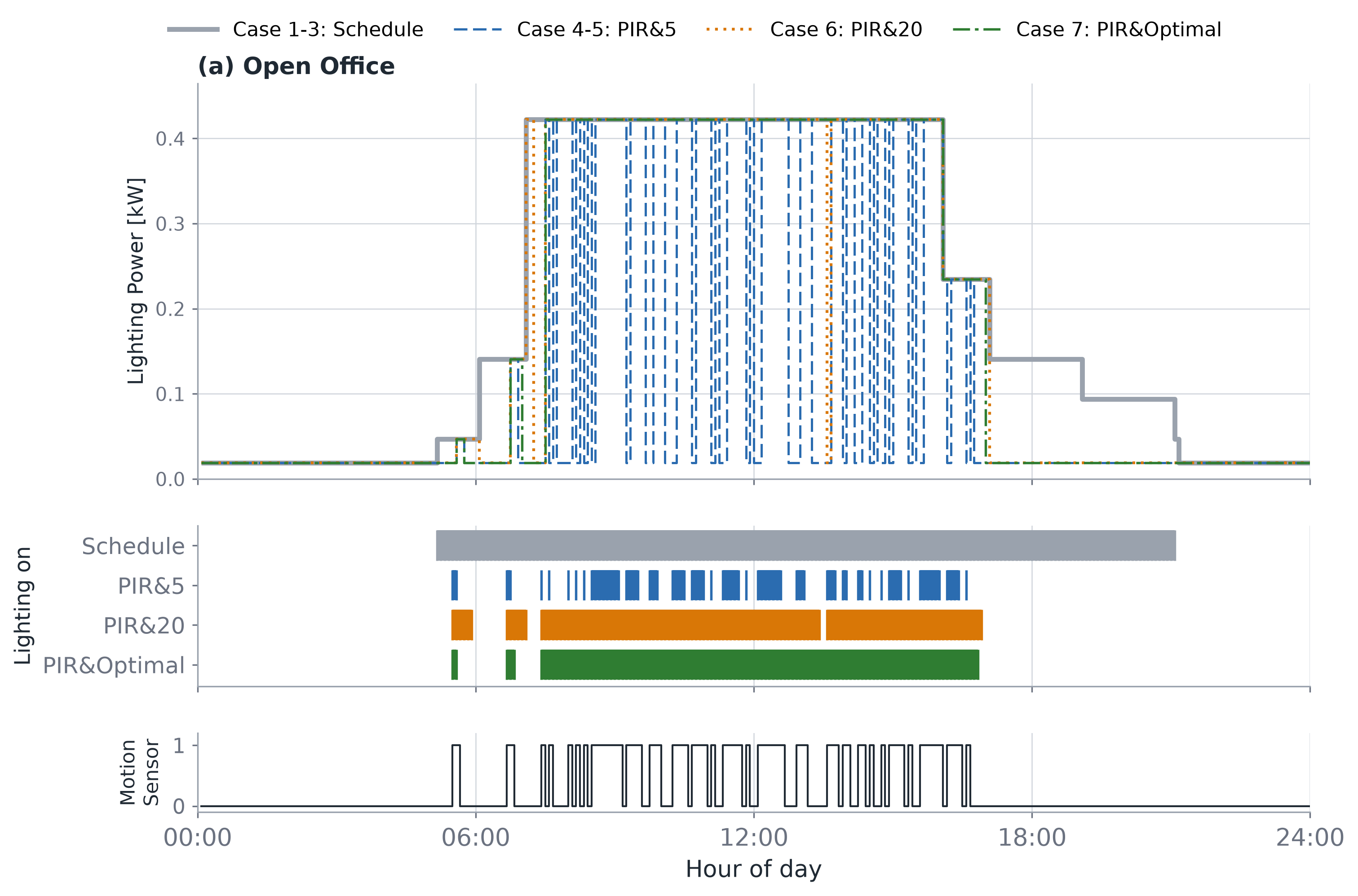
Lighting Control Evaluation
The presented comparisons examine scheduled lighting and PIR-based operation with different hold-time settings, including an optimal hold-time case. A short hold time can reduce unnecessary lighting but increase false-off events; a longer hold time maintains lighting through gaps in motion detection but can increase false-on operation after occupants leave.
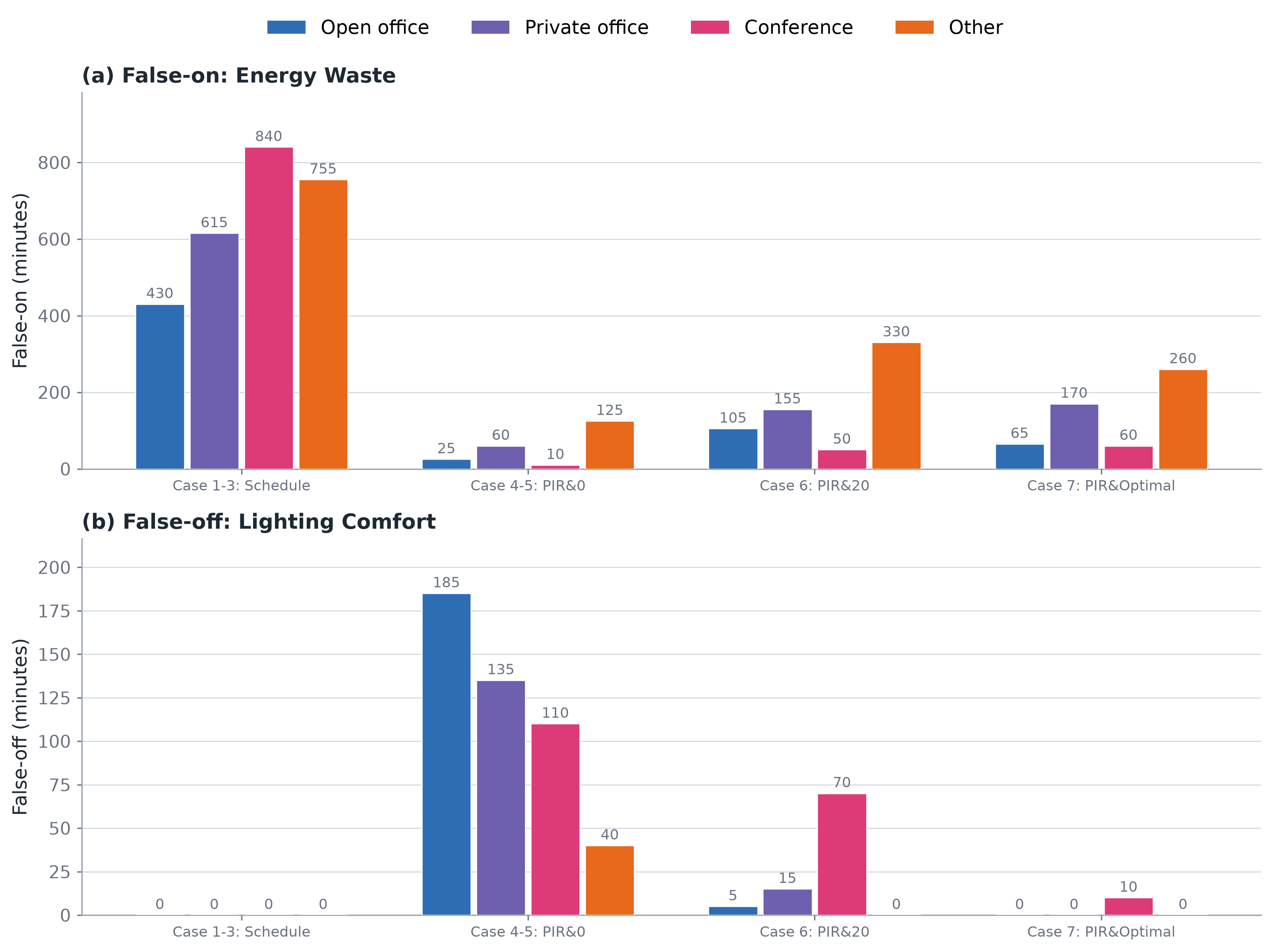
The space-type comparison evaluates false-on and false-off durations in open offices, private offices, conference rooms, and other spaces. These results motivate occupancy-aware predictive control that accounts for differences in occupant behavior and space use, rather than relying on one fixed sensor hold time.
Reference
Differentiable Predictive Control for Occupancy-based Lighting System, Energy and Buildings (In-preparation)
Advanced HVAC Control
Occupancy-based Supervisory Control for Integrated Lighting and HVAC Systems (2026 PNNL Summer Internship)
Overview
This ongoing study investigates occupancy-based supervisory control that integrates lighting and HVAC operation. Differentiable predictive control combines occupancy prediction, lighting on/off and hold-time decisions, supply-air-temperature control, and occupied standby operation to balance energy use with lighting and thermal comfort.
Control Framework
Stochastic room-level occupancy is used to generate PIR sensor data and predict occupied or unoccupied states. The framework combines these signals with a Neural ODE zone-temperature prediction model and a cooling-energy prediction model. Lighting and HVAC controls are evaluated together in an EnergyPlus–Python co-simulation environment.
Case Study
- Location: Portland, Oregon, climate zone 4C (mixed marine).
- Building: a high-fidelity medium-sized office model with rooftop-unit-based multi-zone VAV systems.
- Evaluation period: the cooling season, May through September.
- Comparisons: scheduled control, outdoor-air-temperature reset, ASHRAE Guideline 36, PIR-based occupancy control, and integrated DPC with an optimal hold time.
Energy and Comfort Results
In the presented simulation, integrated DPC uses 15,462 kWh compared with 23,509 kWh for the schedule-based baseline, a 34.2% reduction. The comparison includes cooling, fan, reheat, and lighting energy.
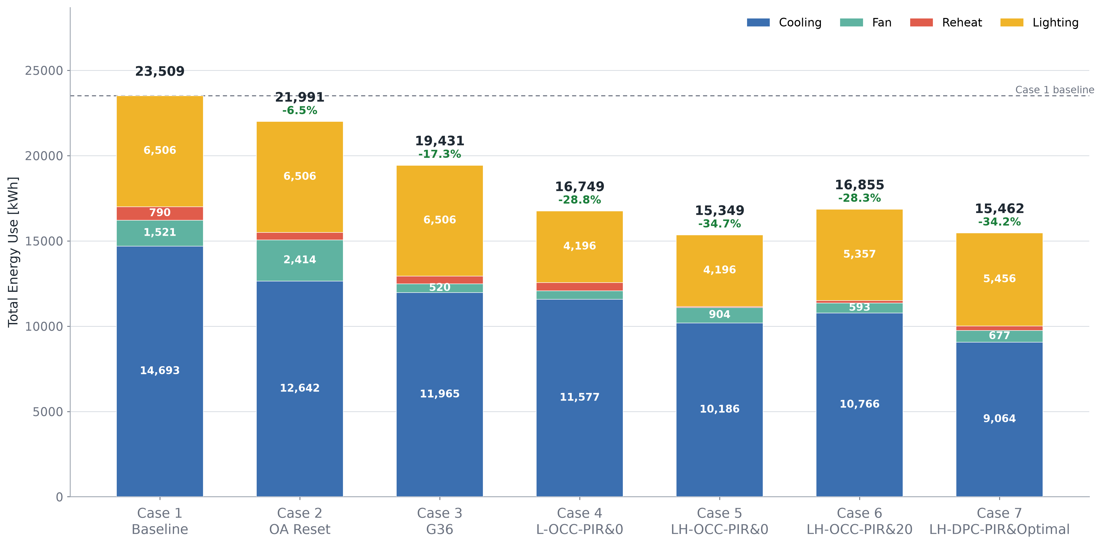
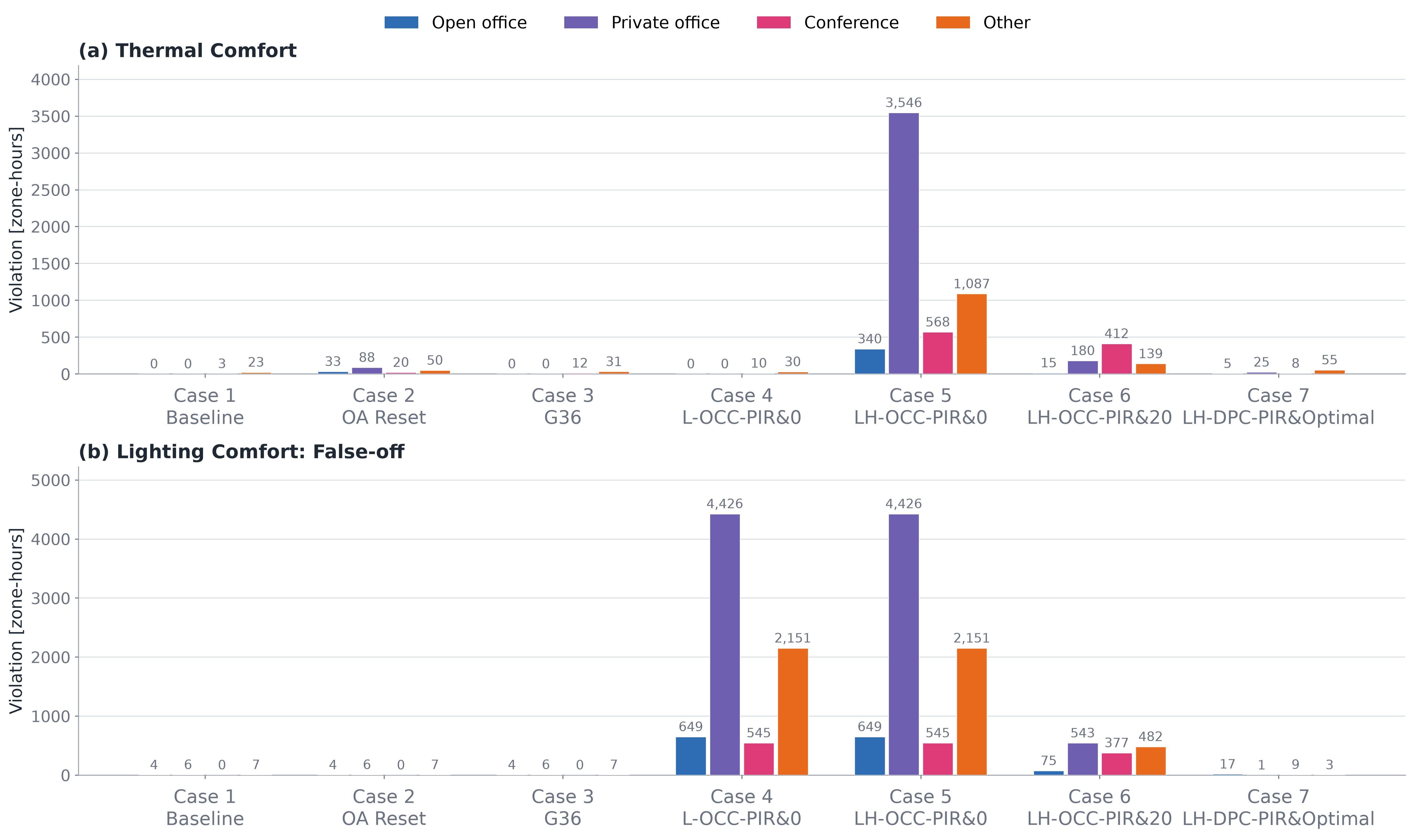
The comfort comparison shows why energy use must be evaluated alongside occupancy sensing errors. Some occupancy-based settings reduce energy use but substantially increase thermal or lighting comfort violations. Integrated DPC maintains low violation levels while reducing energy use; these preliminary results are specific to the presented case study.
Reference
Occupancy-Based Supervisory Control for Integrated Lighting and HVAC Systems (In-preparation)
Grid-interactive Efficient Buildings (GEBs)
AI-Tech Assistant (2024 LBNL Summer Internship)
Overview
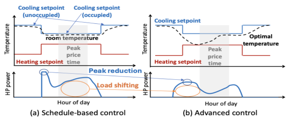
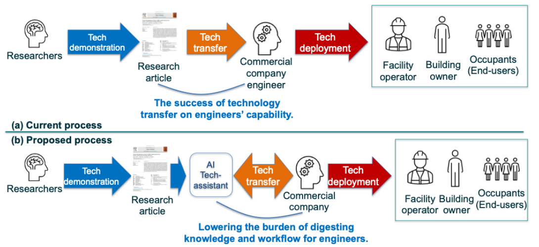
This research develops an AI-Tech Assistant to support the deployment of low-cost model predictive control (MPC) in small and medium commercial buildings. By adjusting HVAC operation, MPC can reduce peak demand and shift electricity use. The study focuses on making the knowledge needed to implement this technology more accessible to engineers and other stakeholders.
Supporting Technology Deployment
Deploying MPC requires more than a control algorithm: practitioners also need to assess site suitability, install the system, and configure its operation. The assistant provides conversational guidance on these tasks, helping users navigate deployment procedures and troubleshoot issues without relying on repeated exchanges with research experts.
Assistant Design and Evaluation
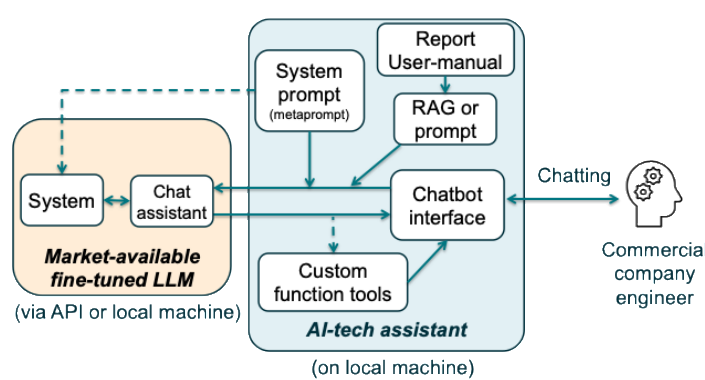
The prototype combines a large language model with deployment-specific instructions, technical context, and custom function tools. Example scenarios examine how it explains MPC concepts, checks site eligibility, and generates configuration templates, while keeping responses within the intended technical scope. These demonstrations illustrate its potential to support technology transfer and identify directions for further development.
Reference
Ham, S. W., Ha, J., Lee, S., and Kim, D. (2025). Development of the AI-Tech Assistant to Transfer Research Outcome Knowledge for Accelerating Low-Cost MPC Technology Deployment. ASHRAE Transactions, 131(Part 1), p. 761. Paper OR-25-C093. https://doi.org/10.63044/w25ham93
Grid-interactive Efficient Buildings (GEBs)
HVAC System
Overview
This research develops differentiable predictive control (DPC) for HVAC demand flexibility in multi-zone commercial buildings. Under time-of-use electricity prices and monthly demand charges, shifting electricity use alone may not reduce the peak demand that determines operating cost. The proposed framework therefore accounts for both energy prices and the maximum demand already recorded within the billing period.
Billing-State-Aware Predictive Control
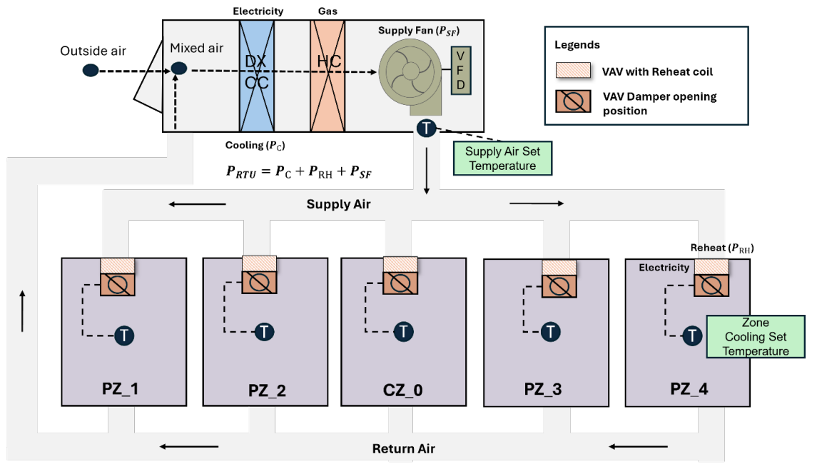
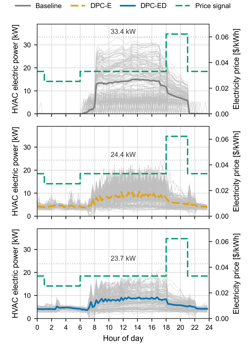
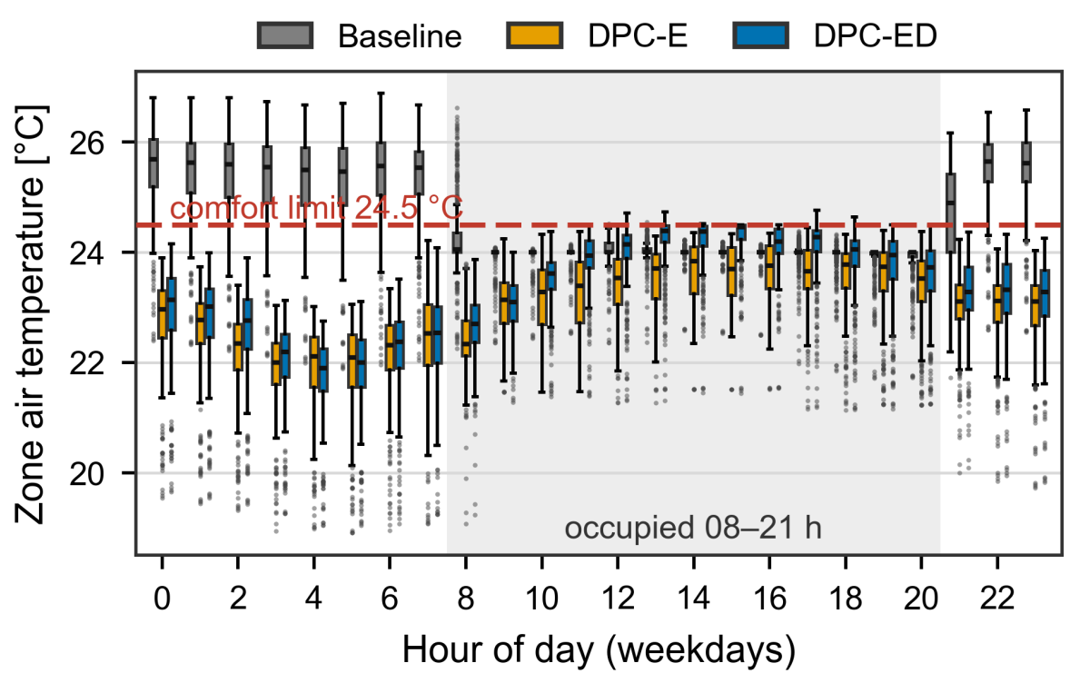
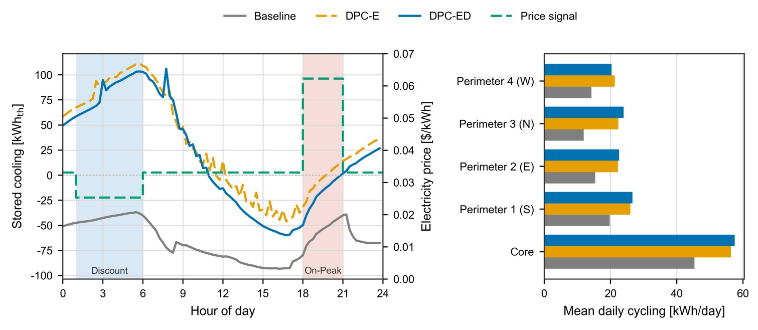
A Neural ODE temperature model and an HVAC power predictor support offline policy training. The trained controller adjusts the cooling temperature setpoint of each zone directly in EnergyPlus without online numerical optimization, while supply-air temperature remains fixed at 12.8 °C. Two formulations are compared: energy-price-responsive DPC (DPC-E) and demand-aware DPC (DPC-ED), which additionally considers demand charges and month-to-date peak demand. Both use the building's thermal mass to shift cooling demand.
Key Results
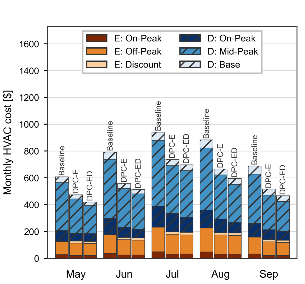
In a five-zone office-building simulation over the May–September cooling season, DPC-ED reduced HVAC operating cost by 31.2%, seasonal peak demand by 29.0%, and occupied-period temperature exceedance by approximately 50% relative to schedule-based control. It also reduced cost by 8.7% compared with DPC-E, with demand-charge reductions accounting for approximately 90% of the savings relative to the baseline.
The policy retained cost and peak-demand reductions when transferred to other floors of the same building without retraining.
Reference
Juwan Ha, Seungmin Lee, Yujin Kim, Sunho Kim, and Soolyeon Cho. Differentiable Predictive Control for Demand Flexibility in Multi-Zone Commercial Buildings, Energy and Buildings (Under review).
Grid-interactive Efficient Buildings (GEBs)
Ice Thermal Energy Storage
Overview
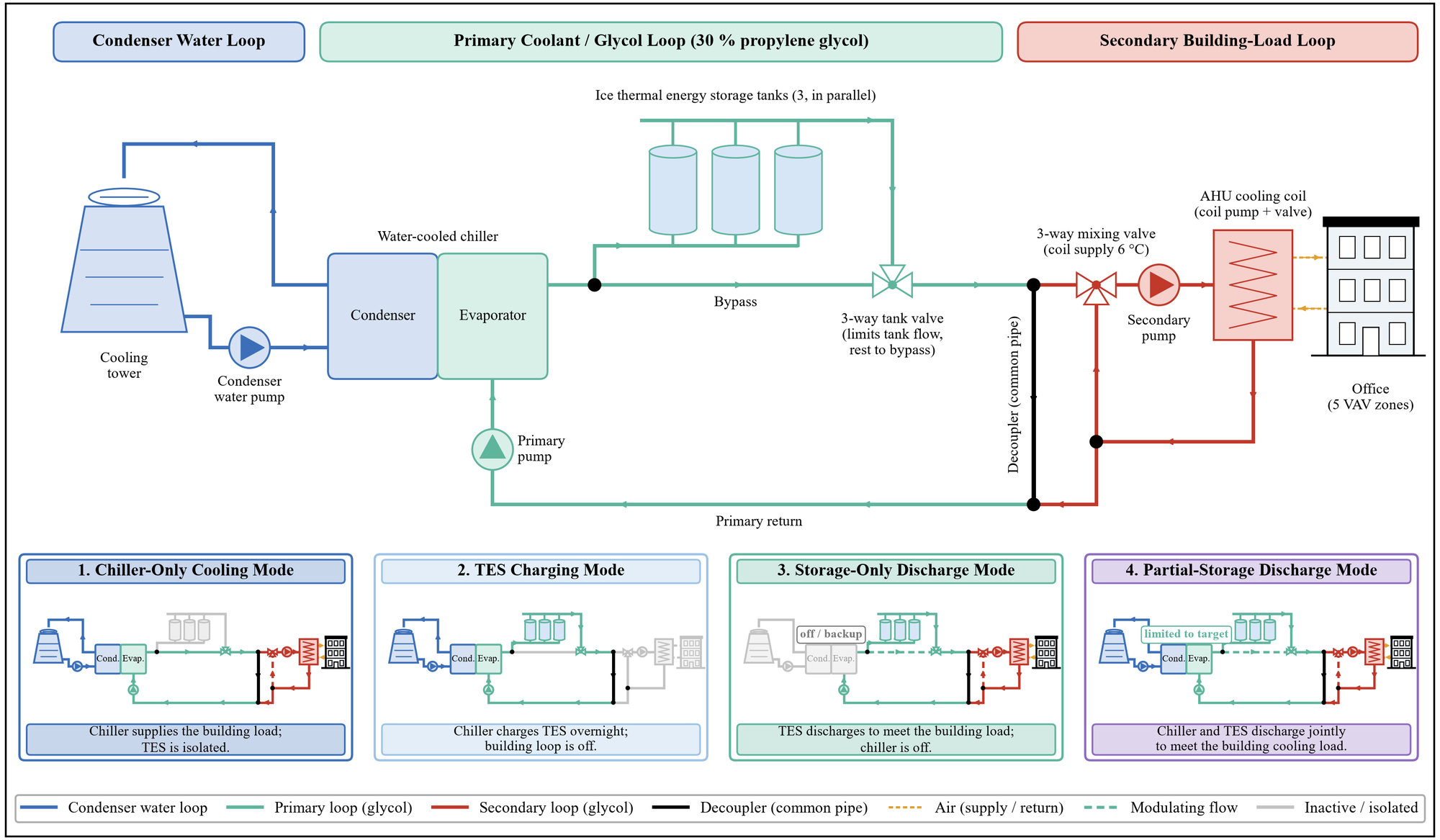
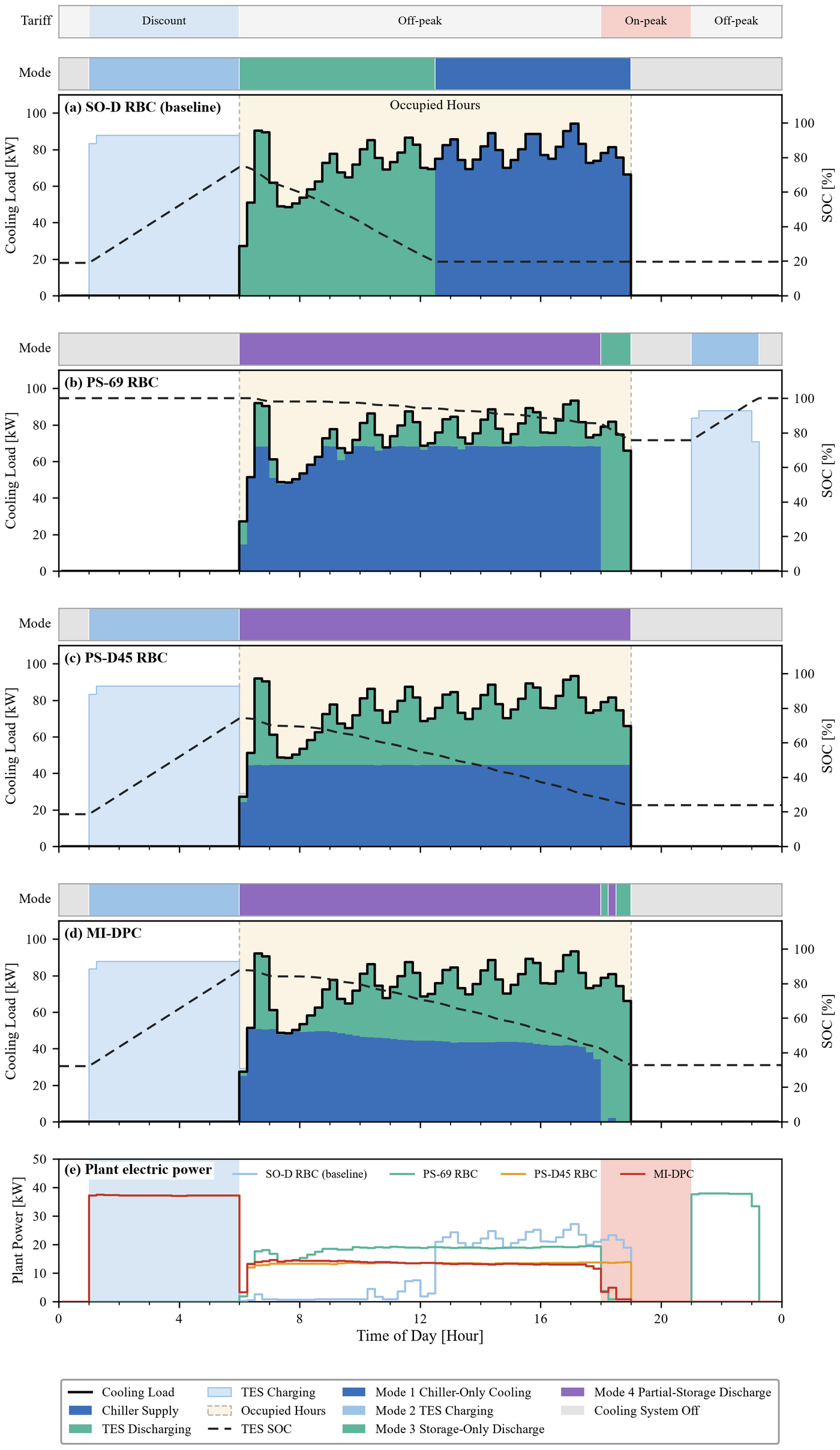
This research develops mixed-integer nonlinear differentiable predictive control (MI-DPC) for a water-cooled chiller plant with ice thermal energy storage (TES) serving a five-zone office building. Under time-of-use (TOU) electricity prices and demand charges, the controller decides every 15 minutes which operating mode to apply—chiller-only cooling, TES charging, storage-only discharge, or partial-storage discharge—together with a continuous chiller cooling target, looking 48 hours ahead (Figure 1).
Physics-Informed Plant Model and Virtual Testbed
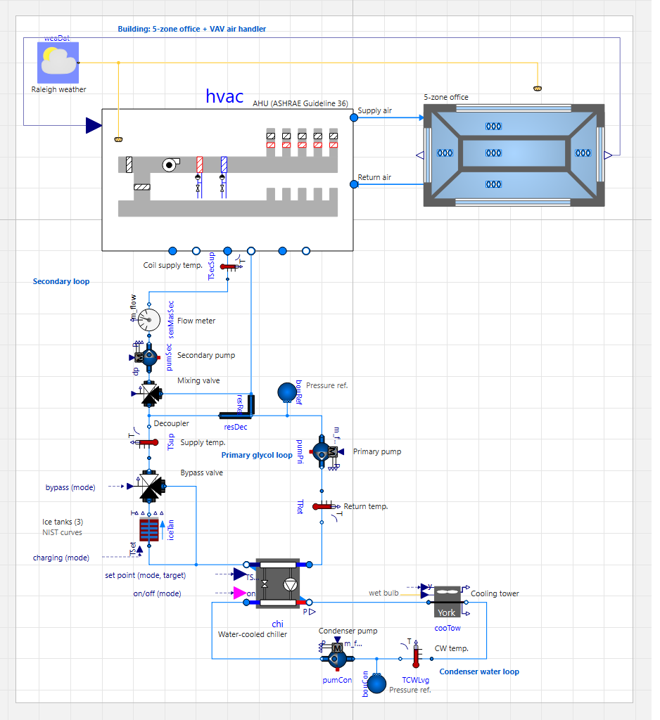
The control policy is trained offline with a physics-informed machine learning plant model: an energy-conserving state-of-charge (SOC) model of the three parallel ice tanks (791 kWhth) and component-level power models of the cooling plant. The trained policy is then evaluated in closed loop on a high-fidelity Modelica testbed coupled to Python through the Functional Mock-up Interface (FMI), which combines the five-zone office and its ASHRAE Guideline 36 VAV air handler with the 130 kWth chiller, ice tanks, pumps, and cooling tower (Figure 2). The case study uses Raleigh, North Carolina weather (climate zone 4A) and a Duke Energy Progress TOU tariff over the May–September cooling season.
Key Results
MI-DPC is compared with rule-based controls (RBC): a storage-only discharge baseline that charges in the discount window (SO-D), and two partial-storage strategies with a fixed chiller target of 69 kWth (PS-69) or 45 kWth (PS-D45). On a representative weekday (Figure 3), MI-DPC charges the tanks in the discount window (01:00–06:00), shares the daytime load between the chiller and the ice with a gradually decreasing chiller target, and serves the on-peak period (18:00–21:00) from ice alone. Daytime plant power stays flat at about 13 kW, and the tanks are drawn down to an SOC of 0.32 by the end of the day, ready to be recharged in the next discount window.
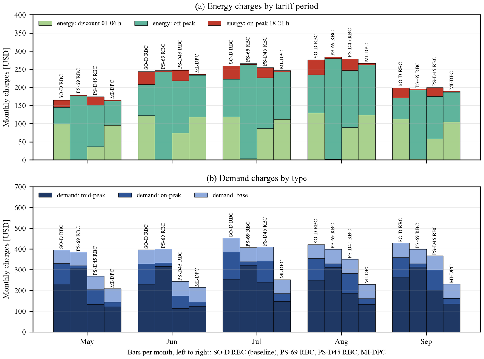
- Season cooling-plant bill: 29.1% lower than the baseline (USD 3,434 → 2,433) and 14.6% lower than the best-performing rule-based strategy (USD 2,850).
- Peak demand: 46% lower mid-peak demand (29.9 → 16.1 kW) and 74% lower on-peak demand (24.5 → 6.3 kW); about 96% of the savings come from demand charges (Figure 4).
- Cooling-plant electricity use is 1.7% higher than the baseline, so the savings come from tariff-aware operation rather than lower energy use. The SOC stayed above its 0.20 lower limit throughout the season.
Reference
Mixed-Integer Nonlinear Differentiable Predictive Control for a Chiller Plant with Ice Thermal Energy Storage, Applied Energy (In-preparation)
Grid-interactive Efficient Buildings (GEBs)
Multi-building Coordinated Control
Overview
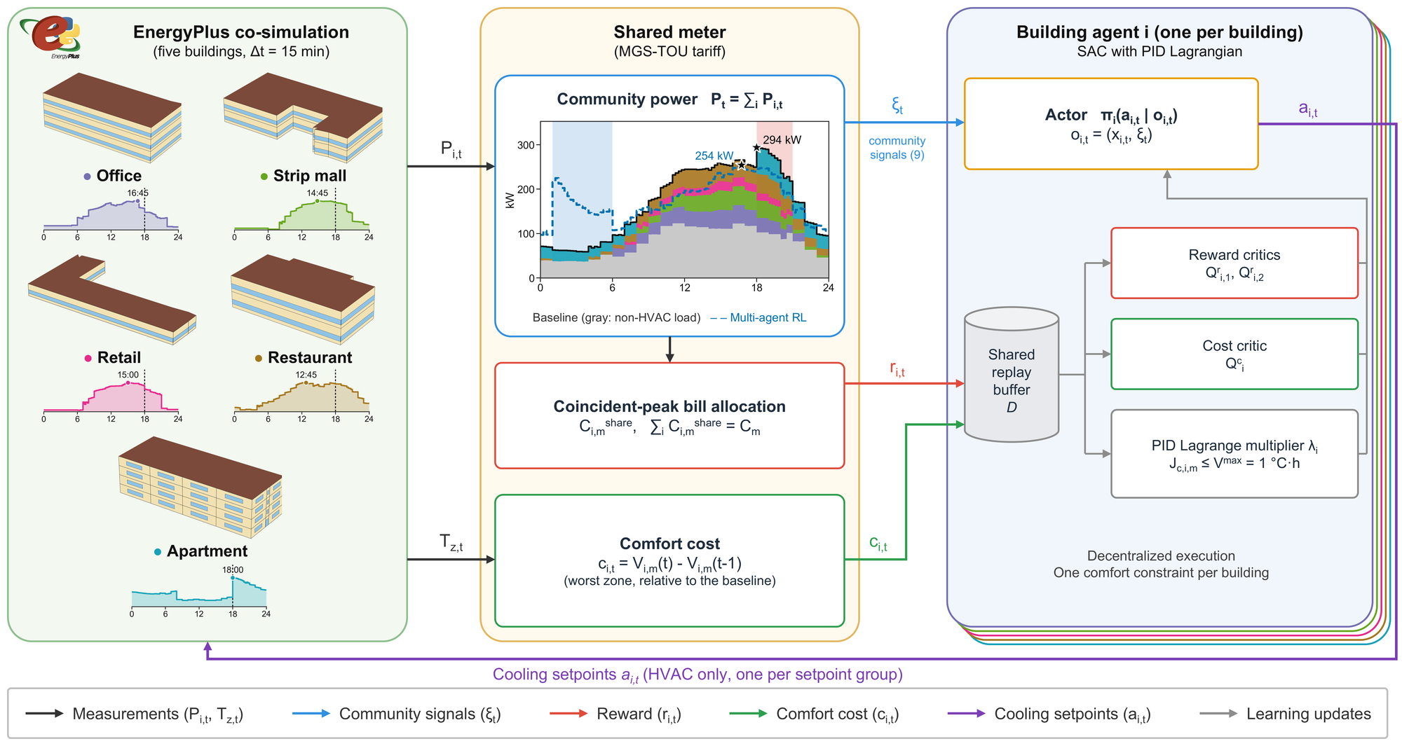
Mixed-use communities offer demand flexibility through their diverse operating schedules, but minimizing each building’s own bill does not necessarily minimize a shared-meter bill, whose demand charges depend on the coincident community peak. This research develops a safe multi-agent reinforcement learning (MARL) framework that coordinates the cooling setpoints of existing HVAC systems in a five-building mixed-use community—an office, a strip mall, a retail store, a restaurant, and an apartment building—without additional storage or generation (Figure 1).
Safe Multi-Agent Reinforcement Learning
Each building agent uses soft actor-critic (SAC) with a PID-updated Lagrange multiplier that keeps its monthly comfort deterioration, relative to schedule-based operation, within a building-specific limit. The agents are rewarded with their coincident-peak shares of the community bill, which sum exactly to the bill under a time-of-use tariff with demand charges. The framework is evaluated in closed-loop EnergyPlus co-simulation at a 15-minute time step for Raleigh, North Carolina: the agents are trained on typical-year weather and evaluated on the actual 2022 (validation) and 2023 (test) weather. It is compared with schedule-based operation (Baseline) and with independent agents trained on their own-meter bills (Single-agent RL).
Key Results
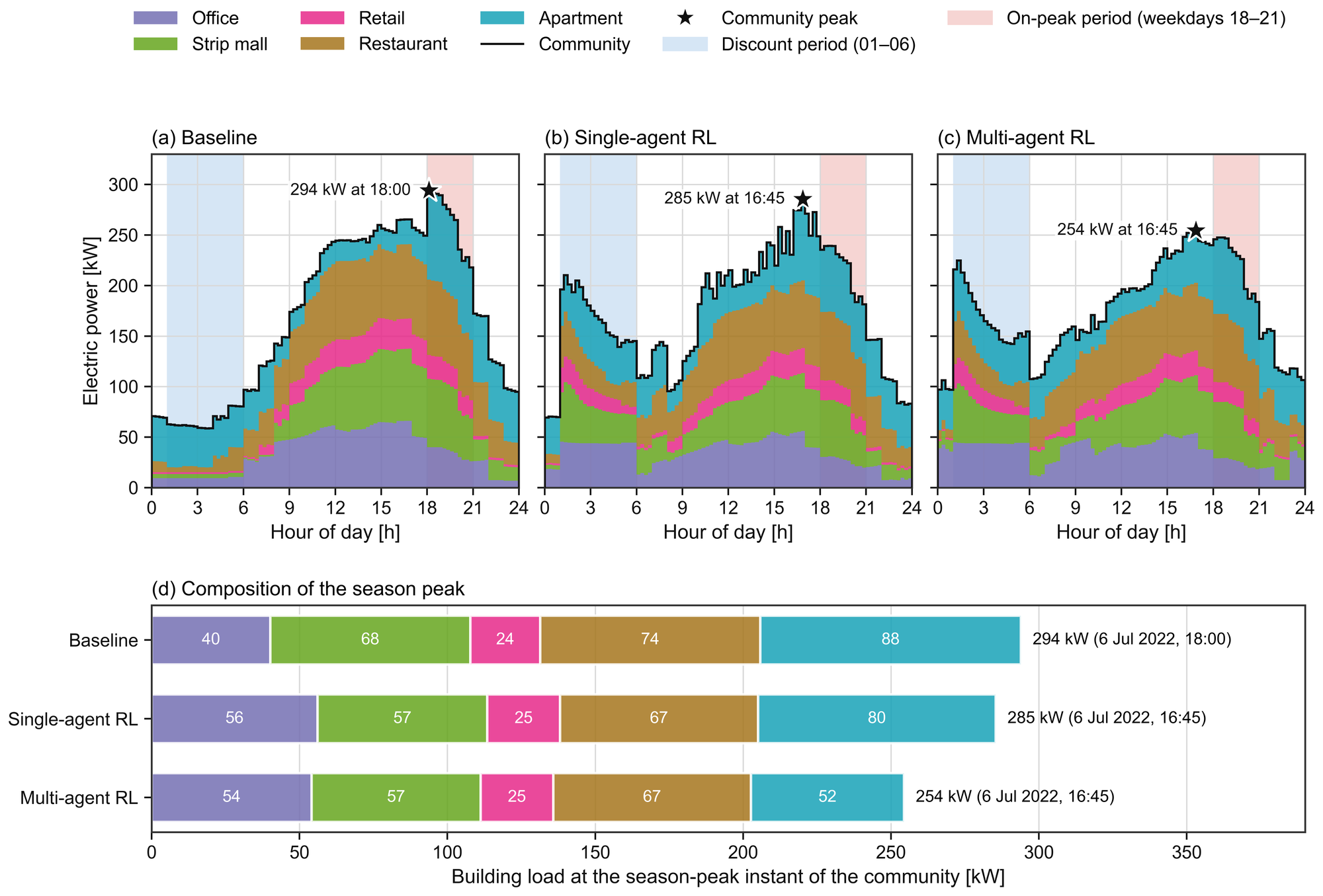
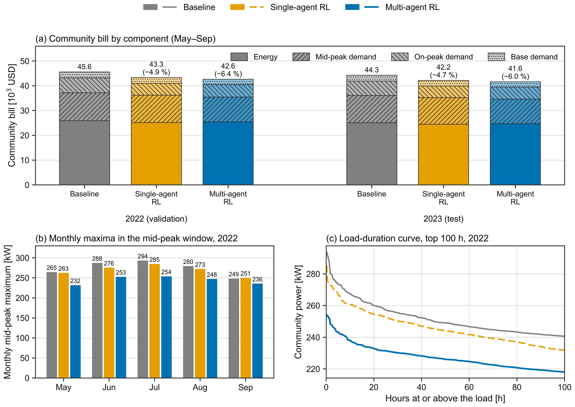
- Community peak: Multi-agent RL reduced the community peak by 13.5% and 10.6% in the validation and test years, versus 2.9% and 1.3% for Single-agent RL. On the representative day, the season peak fell from 294 kW to 254 kW (Figure 2).
- Community bill: 6.4% and 6.0% lower, versus 4.9% and 4.7% for Single-agent RL, mostly through the mid-peak demand charge, while every building met its monthly comfort limit (Figure 3).
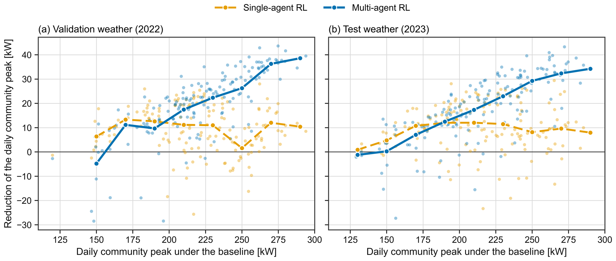
- Daily peaks: the reduction grew with the baseline daily peak, reaching 10–13% on the monthly peak days (Figure 4).
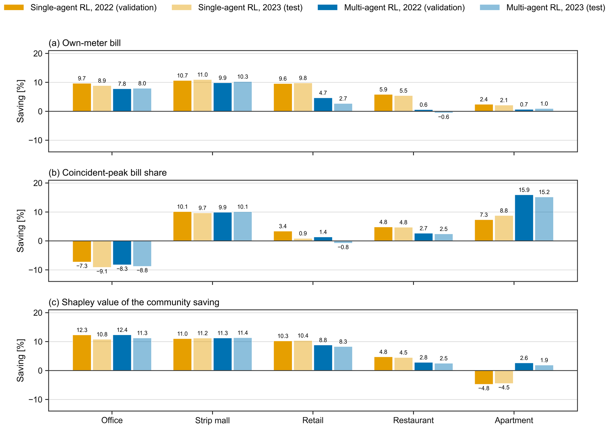
- Trade-offs: the flexibility came from precooling in the discount period, which increased community electricity use by 3.2–3.8% and created a power step at the start of that period. Coincident-peak allocation increased the office’s assigned bill even though a Shapley-value analysis credited it with positive savings, indicating that learning rewards and benefit settlement should be designed separately (Figure 5).
Reference
Juwan Ha, Seungmin Lee, and Soolyeon Cho. Safe Multi-Agent Reinforcement Learning-Based Coordinated Control for HVAC Demand Flexibility in Grid-Interactive Mixed-Use Communities, Energy and Buildings (In-preparation).
Grid-interactive Efficient Buildings (GEBs)
HVAC, PV and Battery
Details coming soon.
Data Center
Air-Cooled Data Centers
Overview
We developed a high-fidelity, physics-based EnergyPlus model of an air-cooled data center (ACDC) with a Computer Room Air Handler (CRAH)-based cooling system. Figure 1 presents the conceptual control sequence diagram of the partial cooling model with a Water-Side Economizer (WSE), while Figures 2 and 3 illustrate the major system components, including the chiller plant, Water-Side Economizer (WSE), and Thermal Energy Storage (TES). Using this framework, we demonstrated reductions in energy consumption, operating cost, and electrical demand. The resulting research contributions have been published in the four peer-reviewed papers listed in the references below, and the developed ACDC platform includes the following system configurations:
- ACDC - Option A: Chiller Plant + WSE
- ACDC - Option B: Chiller Plant + WSE + TES
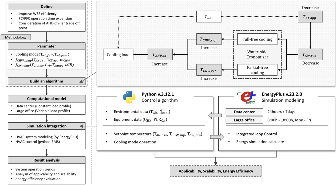
Fig 1. Research flowchart and control sequence conceptual diagram [3]
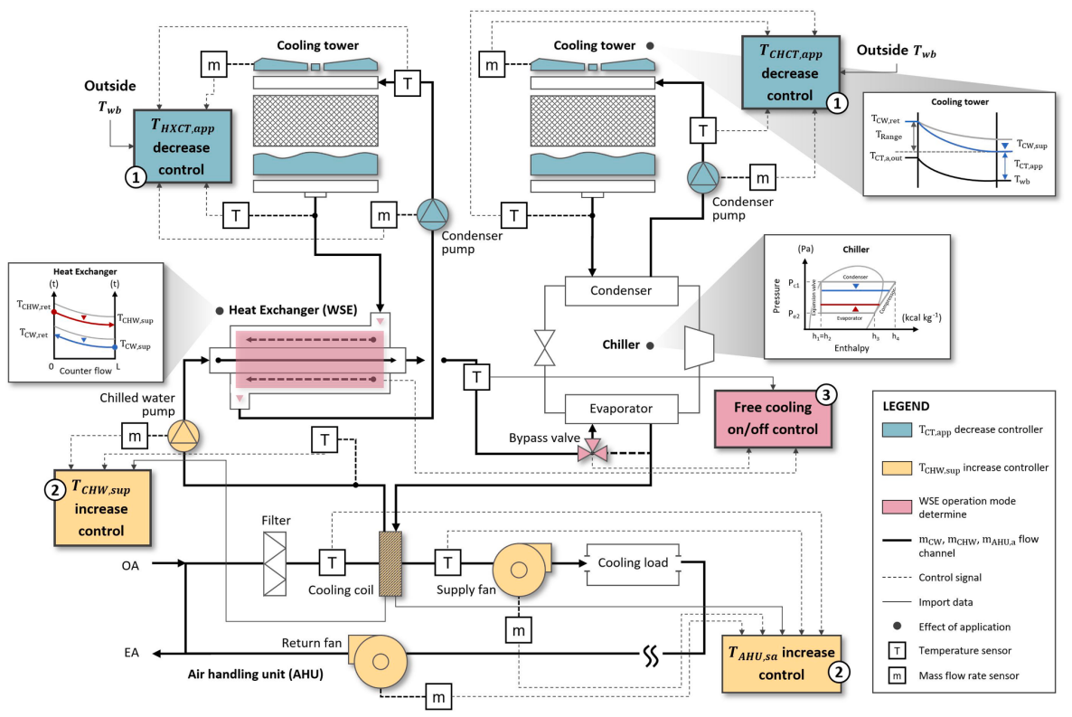
Fig. 2. WSE system schematic diagram [3]
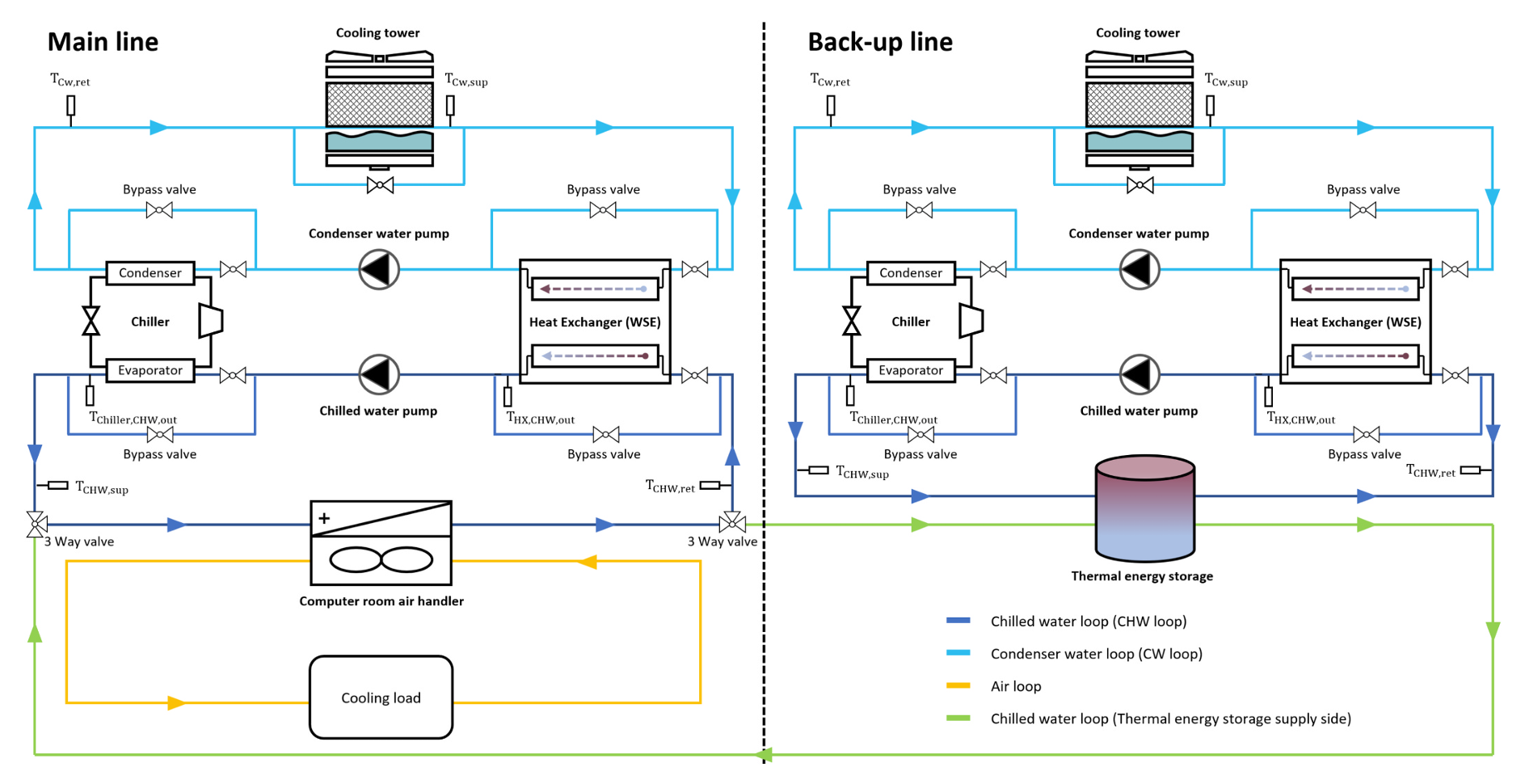
Fig. 3. TES-WSE system schematic diagram [4]
Reference
ACDC- Option A: Chiller Plant + WSE
[1] Yujin Kim, Juwan Ha, Kyung-Soon Park, Young-Hak Song, (2021). A Study on the Energy Reduction Measures of Data Centers through Chilled Water Temperature Control and Water-Side Economizer, Energies, 14(12), 3575, https://doi.org/10.3390/en14123575
[2] Yujin Kim, Kwanghee Kim, Juwan Ha, Young-Hak Song, (2024). Research on a Plan of Free Cooling Operation Control for the Efficiency Improvement of a Water-Side Economizer, (2024). Energies, 17(12), 2804, https://doi.org/10.3390/en17122804
[3] Kwanghee Kim, Yujin Kim, Juwan Ha, Young-hak Song, (2025). Development of an integrated loop control algorithm: Enhancing efficiency and expanding application range for water-side economizers, International Journal of Refrigeration, Vol. 177, 29-39, https://doi.org/10.1016/j.ijrefrig.2025.05.008
ACDC- Option B: Chiller Plant + WSE + TES
[4] Kwanghee Kim, Yujin Kim, Juwan Ha, Young-hak Song., AI-based Model Predictive Control of Chiller Plant with Thermal Energy Storage combined a Water-side Economizer System in Data Centers, Energy and Buildings, 365 (2026), 117668, https://doi.org/10.1016/j.enbuild.2026.117668
Data Center
Liquid-Cooled AI Data Centers
Overview
We aim to develop a high-fidelity, physics-based Modelica modeling framework for liquid-cooled data centers (LCDC) to address the large thermal loads generated by high-density AI server racks. While existing Modelica-based data center models have largely been limited to air-cooled system configurations, this study expands the modeling scope to comprehensively represent both the Facility Water System (FWS) and the Technology Cooling System (TCS) of LCDCs in accordance with the ASHRAE Liquid Cooling Guideline. In particular, to reflect the allowable operating temperature ranges of liquid-cooled server racks, appropriate FWS configurations are established based on the TCS fluid classes defined in the guideline. These configurations include chiller/cooling tower systems, water-side economizers (WSE), and dry coolers, and are classified into the following cases:
- LCDC - Case A: Chiller Only / WSE Partial Cooling Mode
- LCDC - Case B: Cooling Tower Only
- LCDC - Case C: Dry Cooler Only
On the TCS side, the modeling framework incorporates major liquid-cooling components, including Coolant Distribution Units (CDUs), direct-to-chip liquid cooling, rear-door heat exchangers (RDHx), and immersion cooling. This framework is expected to support warmer facility water operation and longer free-cooling hours, thereby improving overall cooling system efficiency and reducing cooling energy use by approximately 20-30%.
2-1) IT and Cooling Load Modeling
Figure 3 presents the overall framework for IT and cooling load modeling. We define the cooling load of our data center models based on tray-level rated IT power for a 2 CPU and 4 GPU configuration (e.g., 6.7 kW) and rack-level rated power (e.g., 120 kW), which are broadly representative of AI training and inference services. Using these rated values, auxiliary loads beyond the servers, and a design-rated Cooling Power Usage Effectiveness (PUE, Total Energy/IT Energy) of 1.2, we estimate the rated IT and cooling loads for a 1 GW-class liquid-cooled data center (LCDC).
We then generate stochastic tray-level IT workloads at the millisecond scale and aggregate them to the rack and Coolant Distribution Unit (CDU) levels. At the cooling interface, direct-to-chip cooling removes heat directly from the primary compute components, while residual rack-level air-side heat is captured through rear-door heat exchangers (RDHx).
These aggregated IT workloads are then translated into minute-resolution cooling loads by accounting for the thermal inertia of the liquid-cooling loop, fluid transport delay, and the response characteristics of the cooling control system. Because the cooling infrastructure responds more slowly than the millisecond-scale IT workload, the resulting plant-level demand is naturally smoothed over time. The resulting composite load curve therefore captures not only the IT load itself, but also cooling tower fans, condenser-water-system (CWS) pumps, chillers, facility-water-system (FWS) pumps, technology-cooling-system (TCS) pumps, Coolant Distribution Units (CDUs), RDHx fans, and other relevant auxiliary loads, enabling a smoother and more physically realistic representation of the coupled IT-cooling dynamics.
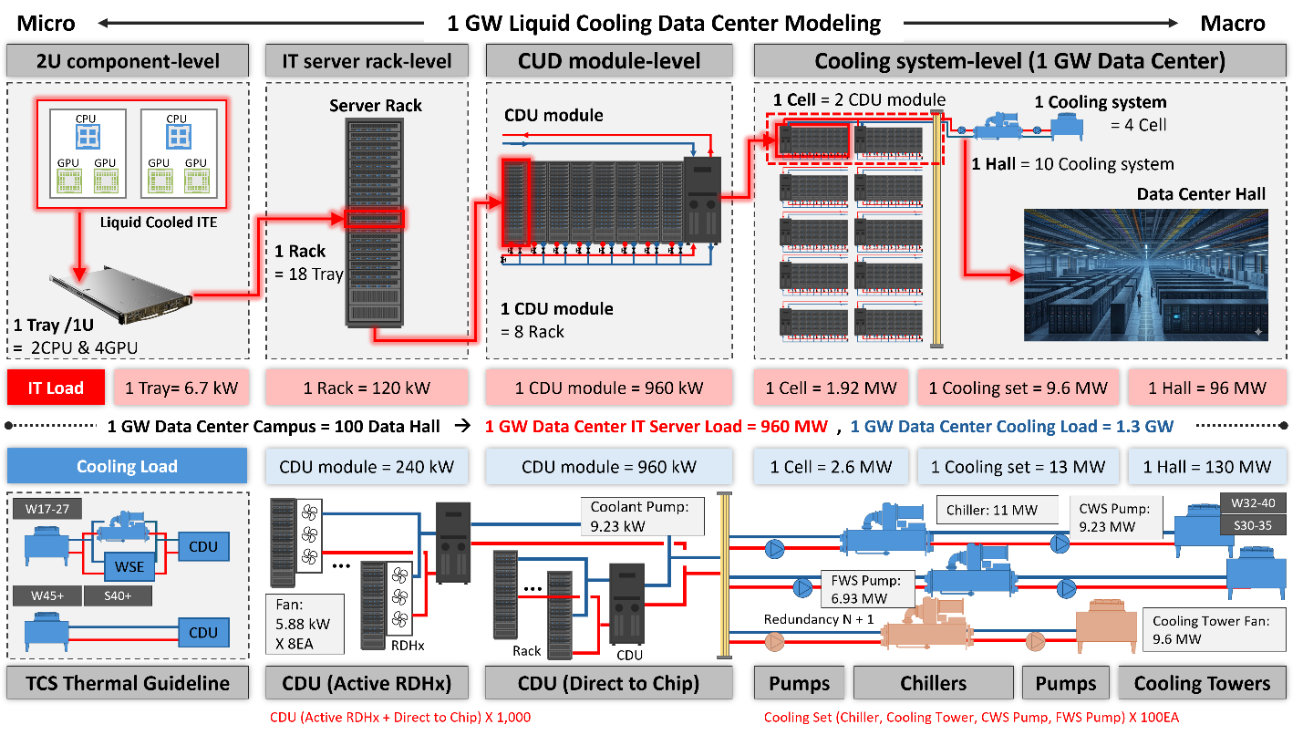
Figure 3. IT and Cooling Load Modeling
2-2) Liquid Cooling Data Center System
On the TCS side, the coolant distribution unit (CDU) is modeled to represent a hybrid cooling architecture in which heat generated by the primary compute components, such as CPUs and GPUs, is removed directly through cold-plate-based direct-to-chip cooling, while residual rack-level air-side heat is captured through active rear-door heat exchangers (RDHx). This enables a more realistic representation of the combined liquid-cooling and air-side supplemental cooling characteristics of AI data centers.
At Data Hall level, each system is designed with N+1 redundancy to ensure stable and reliable operation, and the potential application of thermal energy storage tanks is also considered to enhance emergency response capability and provide additional operational flexibility.
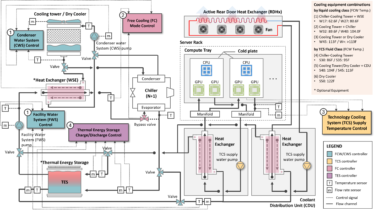
Figure 4. System Overview of the Liquid Cooling Data Center
Reference
IT and Cooling Load Modeling
[1] NVIDIA Corporation, NVIDIA DGX GB Rack Scale Systems User Guide, Mar. 3, 2026.
[2] Vertiv Group Corp., Vertiv(TM) Liebert(R) XDU 1350 - Coolant Distribution Unit (CDU), doc. no. MKA4L0UKXDUDS1350, rev. 1- (R01/23), 2023.
[3] Vertiv Group Corp., Vertiv(TM) Liebert(R) DCD: Energy Efficient Cooling for High Density Applications, doc. no. MKA4L0UKDCD, rev. R04/22, 2022.
[4] Trane, High-Efficiency Cooling for the 1 GW AI Factory: Reference Design #502, High Condenser Temperature System Design featuring CenTraVac(R) Simplex
Real-world Dataset for LCDC Model Validation
M100 dataset 1 is a real-world open dataset collected from Marconi100, a Tier-0 supercomputer at CINECA, and can serve as a valuable reference dataset for validating LCDC (Liquid Cooling Data Center) models. It includes not only node-level measurements from more than 980 computing nodes, such as core load, temperature, frequency, memory activity, CPU power, fan speed, and GPU utilization, but also system-level information covering the liquid cooling infrastructure, air-conditioning system, power supply units, workload manager statistics, job-related information, system alerts, and weather data. Covering the period from March to December 2020, the dataset is stored as a partitioned Parquet dataset organized by year_month, plugin, and metric, and distributed as monthly tarballs, making it well suited for analyzing the thermal and operational behavior of large-scale liquid-cooled data centers and for model validation purposes.
[5] Andrea Borghesi, Carmine Di Santi, Martin Molan, Mohsen Seyedkazemi Ardebili, Alessio Mauri, Massimiliano Guarrasi, Daniela Galetti, Mirko Cestari, Francesco Barchi, Luca Benini, Francesco Beneventi, and Andrea Bartolini. (2023). M100 dataset 1: from 20-03 to 20-12 (1.0.0) [Data set]. Zenodo. https://doi.org/10.5281/zenodo.7588815
Data Center · Liquid-Cooled AI Data Centers
Energy Efficiency Strategies
Overview
This study applies differentiable predictive control (DPC) to the hybrid liquid cooling system of an NVIDIA GB200 NVL72 pod, in which cold plates and active rear-door heat exchangers (RDHx) are served by two coolant distribution units (CDUs) and a chiller plant with a water-side economizer (WSE). Facility-side cooling plants are usually operated with fixed set points that ignore the weather, the IT load, and the coupling between the rack-side and facility-side loops. The DPC instead sets three plant set points every hour—the chilled-water supply temperature, the condenser-water supply temperature, and the condenser-water flow ratio—within thermal limits, using a 6-hour forecast horizon.
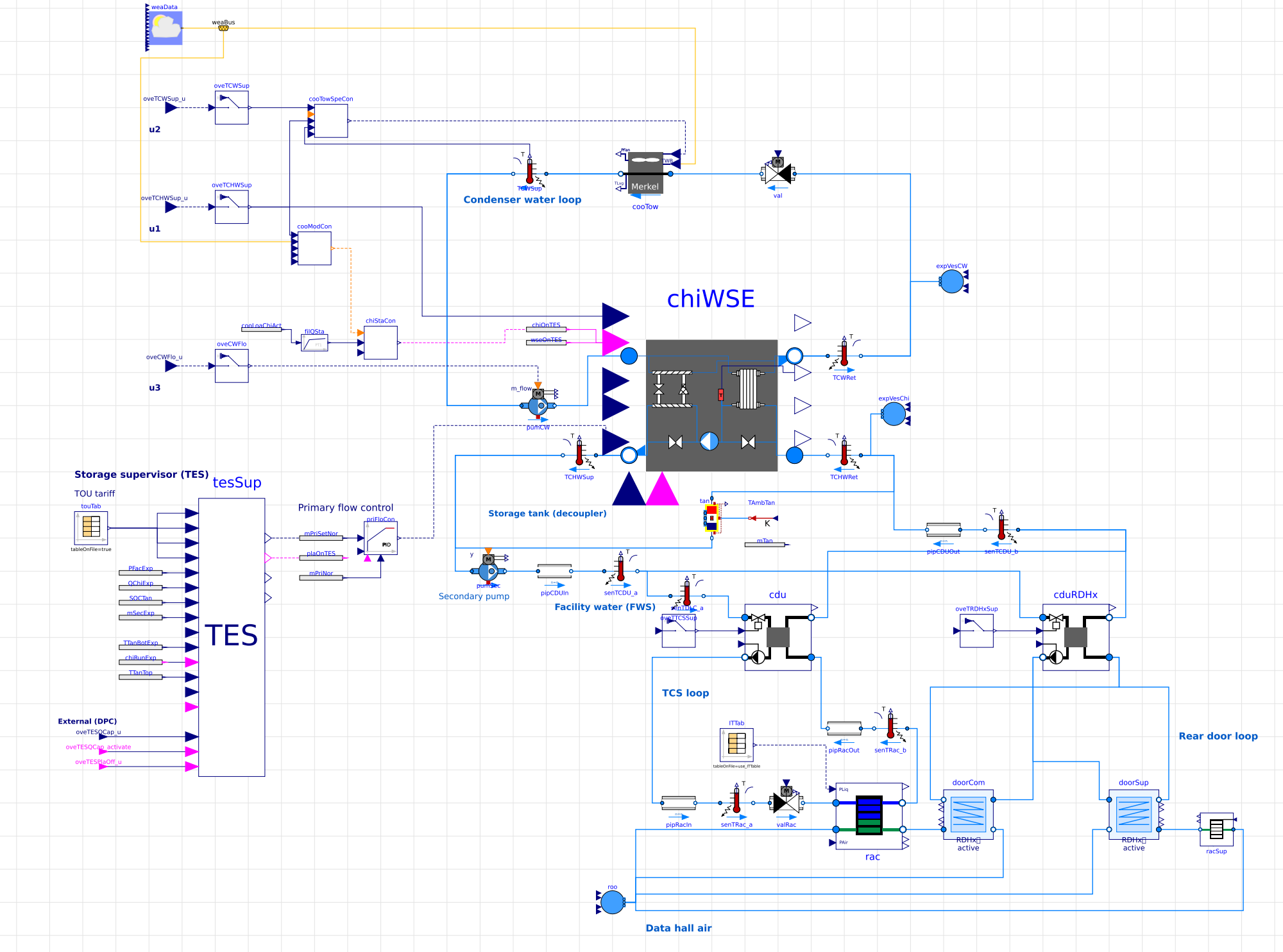
Modelica System Model
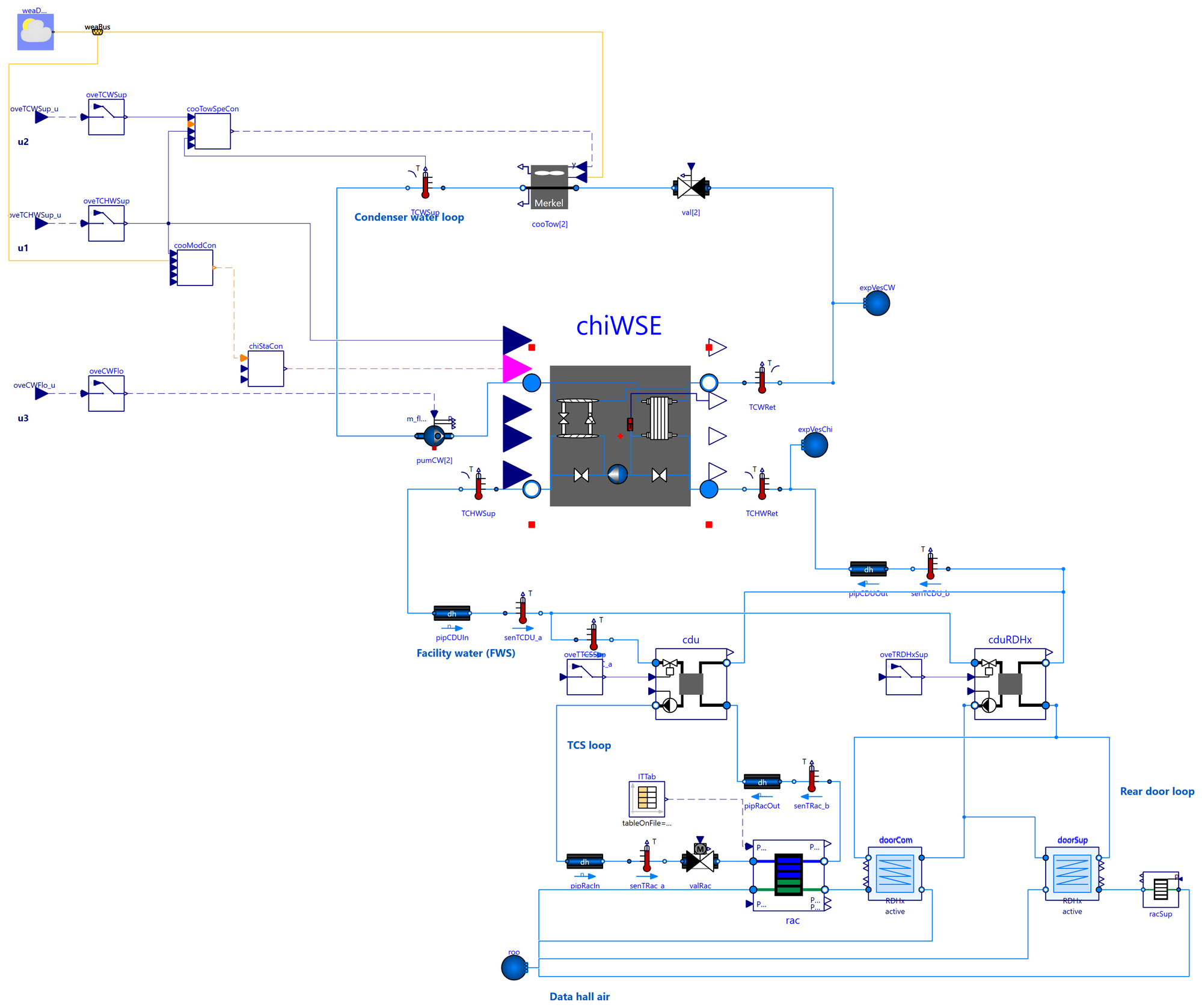
A Modelica model built on the Buildings Library serves both as the emulator that generates training data and as the virtual testbed for annual closed-loop evaluation (Figure 1). A neural state-space model of the plant and a PatchTST IT-load forecast are learned from the emulator data, and the explicit DPC policy is then trained offline through differentiable closed-loop rollouts.
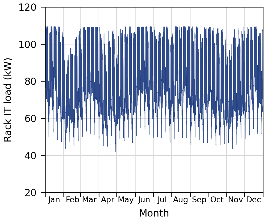
The IT load is based on one-minute power profiles of generative AI inference workloads measured by the National Laboratory of the Rockies (NLR) at 20, 40, 60, and 80% utilization (Vercellino et al., 2026). These profiles are blended according to each day’s utilization to form a one-year time series centered on an annual mean utilization of 60%, with random monthly and daily variations (Figure 2).
Key Results
In a one-year simulation for Raleigh, North Carolina, the DPC was compared with the Buildings Library baseline control:
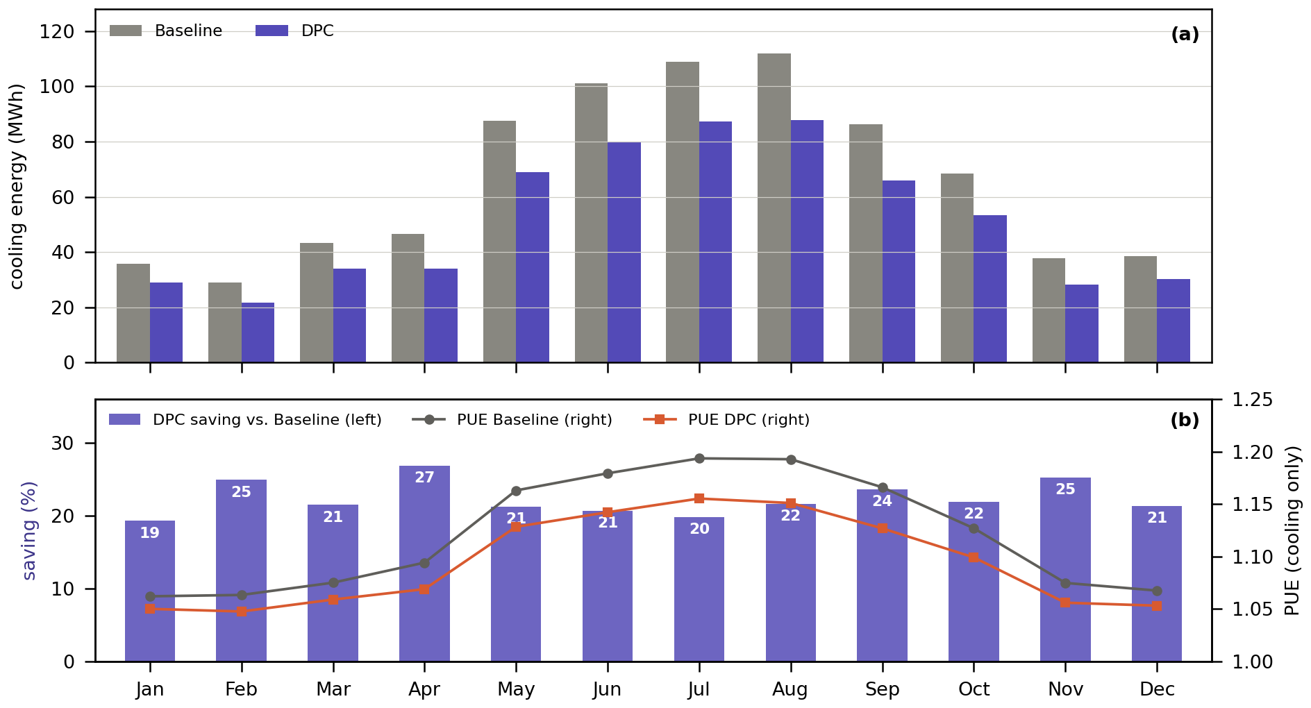
- Annual cooling energy fell by 21.9% (794.6 → 620.2 MWh), about 2.4% of the total facility energy including IT, and the cooling-only PUE dropped from 1.123 to 1.096, with no thermal or equipment limit violations in the 5-minute records.
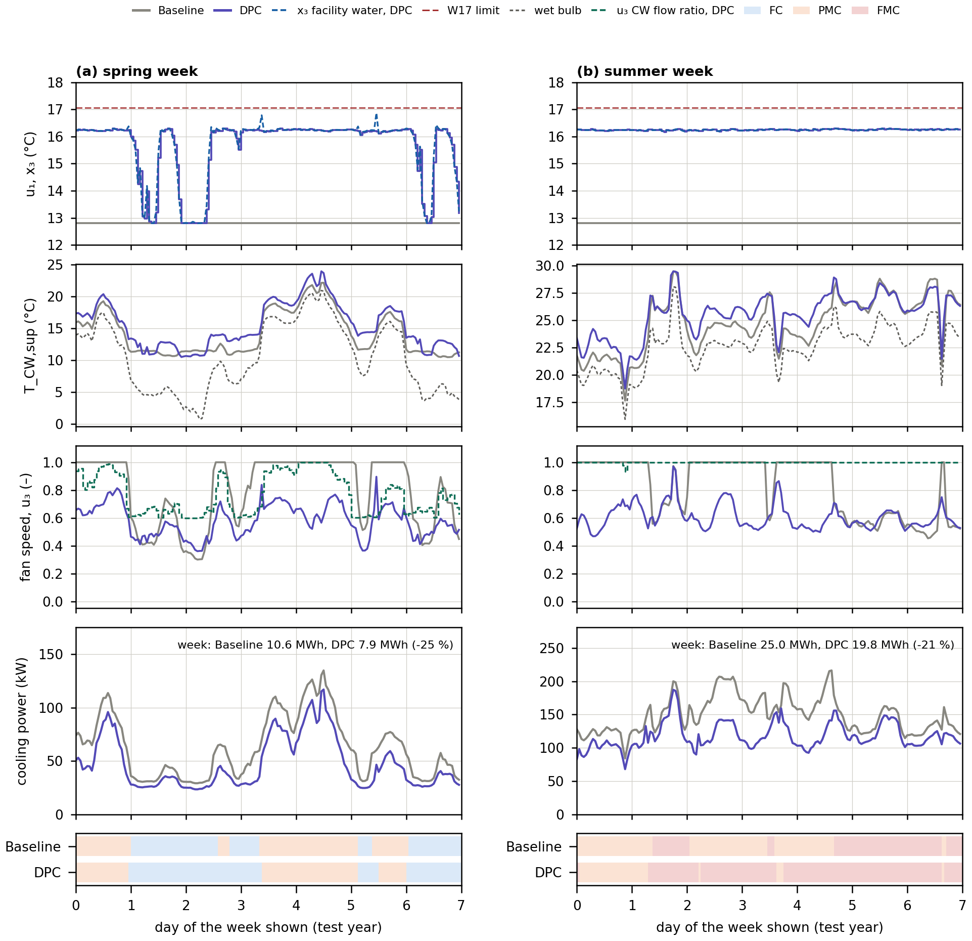
- Most savings came from the cooling-tower fans (−60%), largely by avoiding the baseline’s full-speed fan rule, and from the chillers (−22%): the DPC raises the chilled-water set point close to the facility-water limit, increasing the chiller COP from 7.45 to 10.07 and extending free-cooling hours (Figure 3).
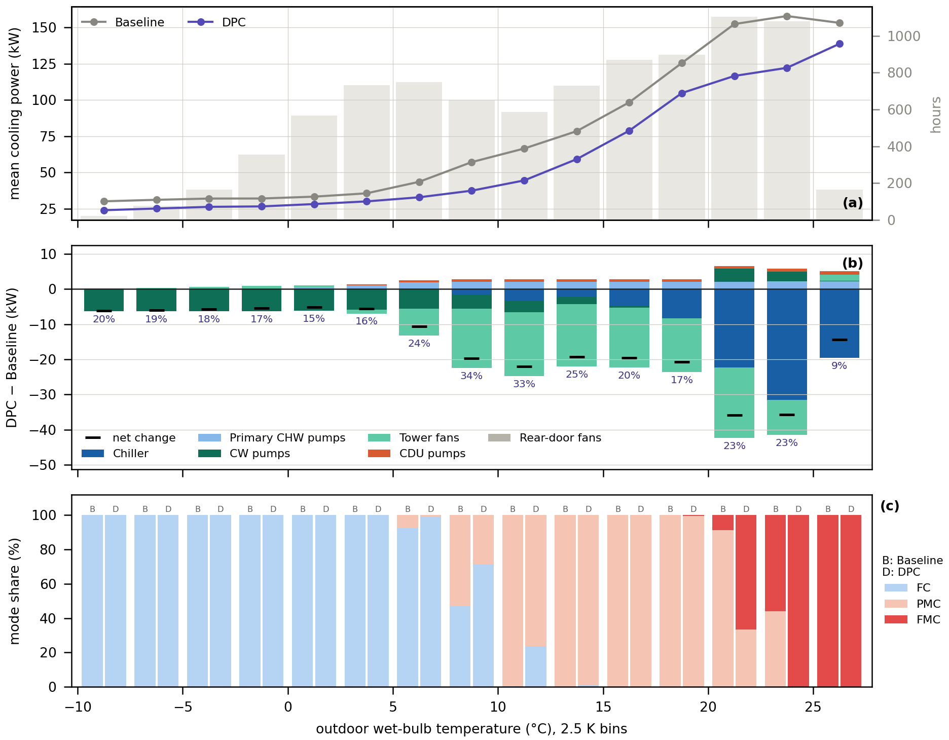
- Savings were largest (33–34%) in the 7.5–12.5 °C wet-bulb transition range (Figure 4), and monthly savings ranged from 19% to 27% (Figure 5). The facility-water safety margin governed the trade-off between savings and constraint compliance.
Reference
Differentiable Predictive Control for Energy-Efficient Liquid Cooling Systems in AI Data Centers (In-preparation)
Data Center · Liquid-Cooled AI Data Centers
Demand Flexibility Strategies
Modelica System Model
Data Center · Liquid-Cooled AI Data Centers
GPU Inference Service Load Generation
Overview
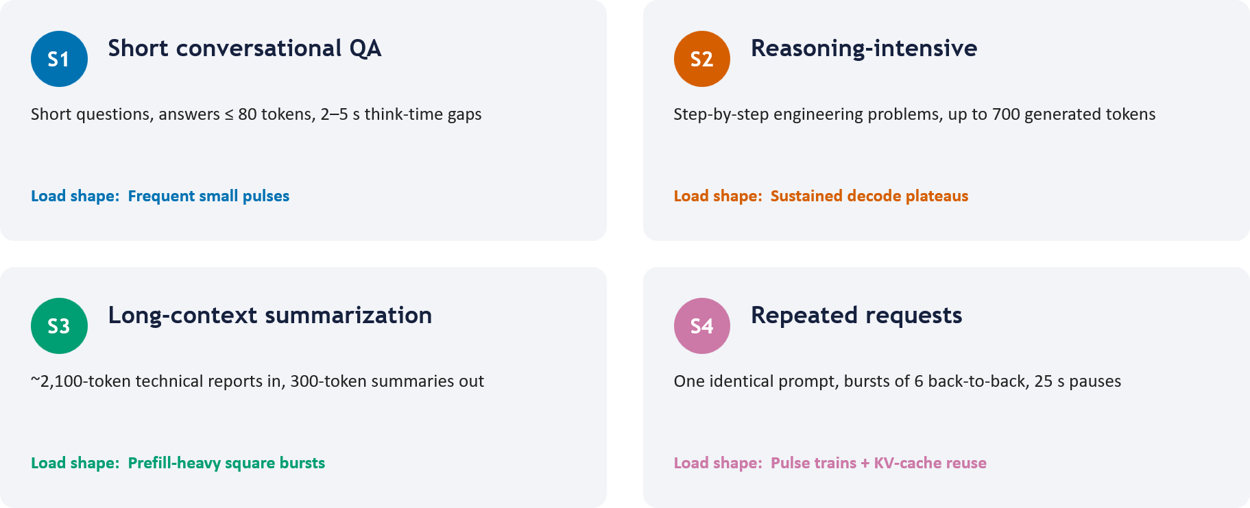
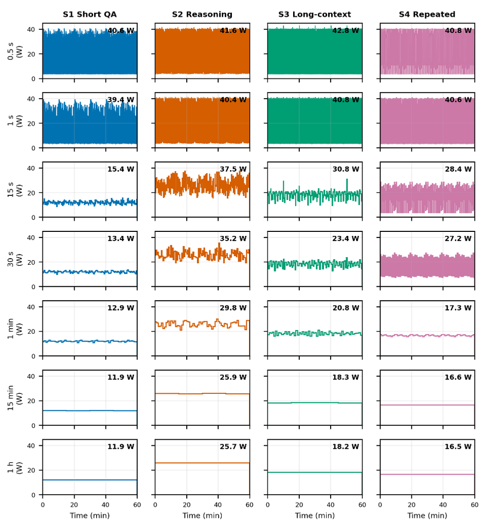
With the rapid growth of large language model (LLM) services, the power and thermal behavior of GPUs in AI data centers increasingly depends on how they are used. This study characterizes how GPU power and temperature patterns change across four representative LLM inference services: (S1) short conversational question answering, (S2) reasoning-intensive generation, (S3) long-context summarization, and (S4) repeated burst requests. Future work will model the transient response to rapid GPU temperature changes in Modelica to evaluate the stability of the cooling system.
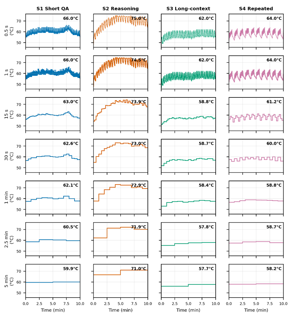
Reference
Juwan Ha, Seungmin Lee, Yujin Kim, Jae Yoon Byun, and Soolyeon Cho. Beyond Static IT Loads: Service-Driven Dynamic Thermal Behavior of LLM Inference in AI Data Centers (Under review).
NC State Campus Building and District System Modeling
District Cooling Systems with Chilled-Water Thermal Energy Storage
Overview
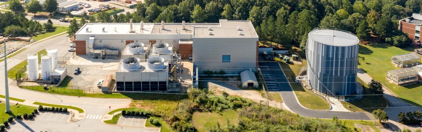
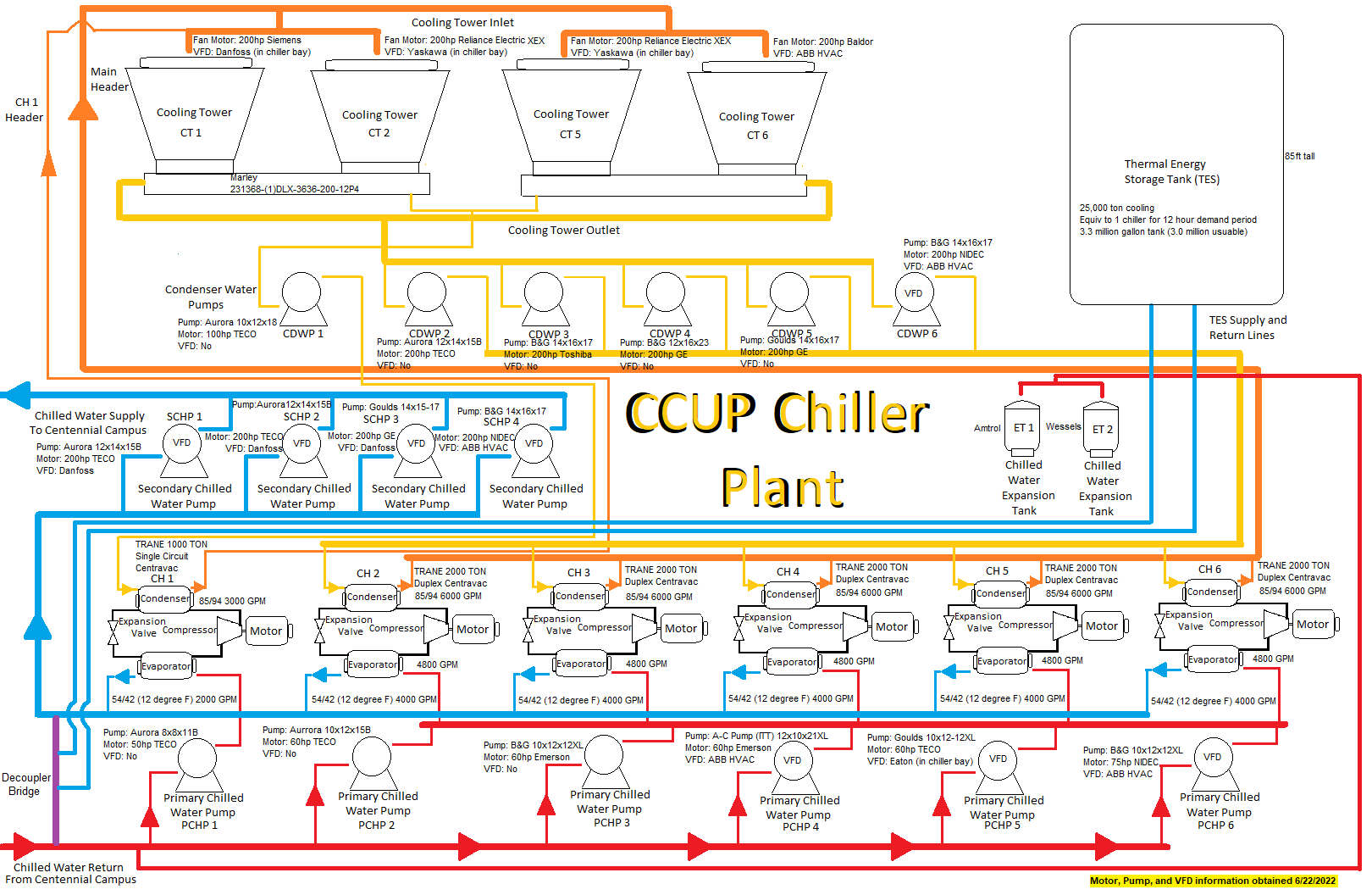
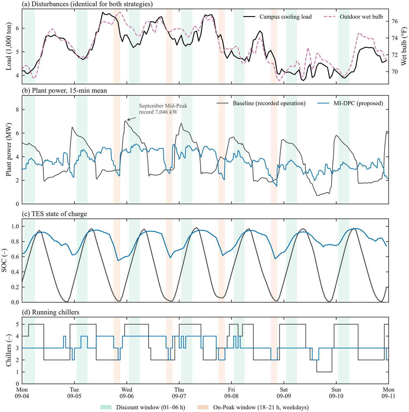
This research develops mixed-integer nonlinear differentiable predictive control (MI-DPC) for the Centennial Campus Utility Plant (CCUP), which supplies chilled water to the campus with five 2,000 RT centrifugal chillers and a 25,000 ton·h (87.9 MWhth) stratified chilled-water TES tank (Figures 1 and 2). More than 60% of the plant’s electricity bill comes from demand charges, yet the plant follows a fixed schedule that does not consider when those charges are set. Under a time-of-use tariff with demand charges (Duke Energy Progress LGS-TOU), MI-DPC decides every hour how many chillers to run and how much to charge or discharge the tank, looking 48 hours ahead.
Calibrated Modelica Plant and Closed-Loop Evaluation
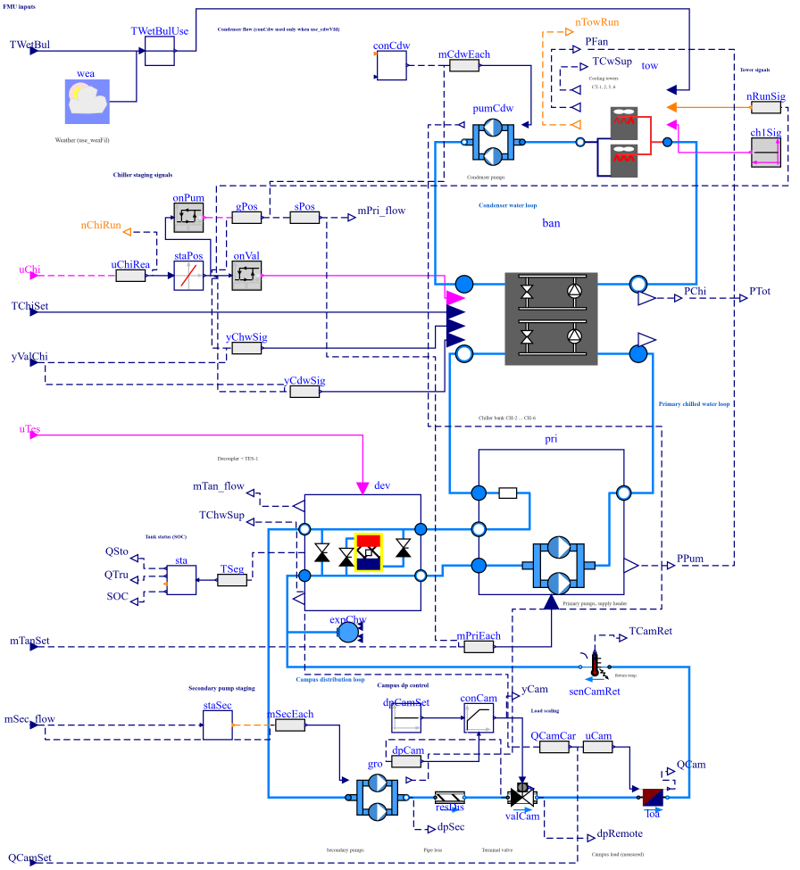
The plant is modeled in Modelica from as-built drawings and calibrated against measured data from July–September 2023 to meet ASHRAE Guideline 14 (Figure 3). The calibrated model is exported as a Functional Mock-up Unit (FMU), and a Python controller overrides its chiller commands and tank flow every hour. The policy is trained on a differentiable grey-box twin of the plant, with campus cooling-load forecasts from a PatchTST model.
Baseline vs. MI-DPC
The baseline is the plant’s recorded operation, a schedule-based storage-priority control: the tank is charged every night (22:00–09:00) and discharged first during the day, until it is nearly empty by the evening. Both strategies run on the same FMU with the same weather, campus load, and 15-minute billing over July–September 2023 (2,184 h). In the September test week (Figure 4), the baseline’s night charging starts before the 01:00–06:00 discount window, so the charging power sets the month’s mid-peak demand record of 7,046 kW. MI-DPC instead keeps the tank state of charge between 0.55 and 0.97 and runs two to four chillers, keeping 15-minute plant power at or below 5,077 kW.
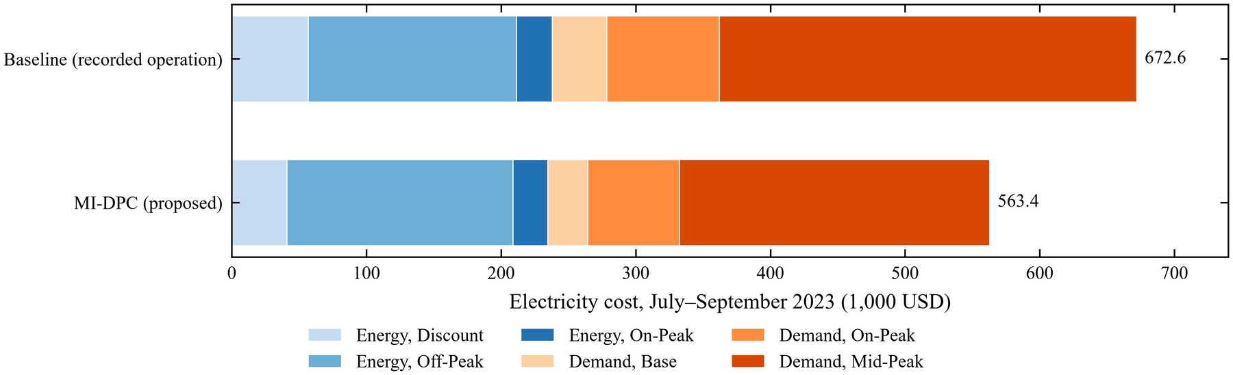
- Quarterly electricity cost: 16.2% lower than the baseline (USD 672,599 → 563,363), and 17.7% lower in September, the month not used for training or policy selection.
- Demand charges: 24.4% lower, accounting for 96.9% of the savings; monthly mid-peak demand records fell by 22.8–29.0% (Figure 5).
- Cooling service: hours with campus supply temperature above 44 °F (6.7 °C) fell from 234 to 4.
Reference
Juwan Ha, Seungmin Lee, Yujin Kim, and Soolyeon Cho. Differentiable Predictive Control for Grid-Interactive District Cooling Systems with Chilled-Water Thermal Energy Storage, Applied Energy (In-preparation).
NC State Campus Building and District System Modeling
Centennial Campus Building Modeling
Overview
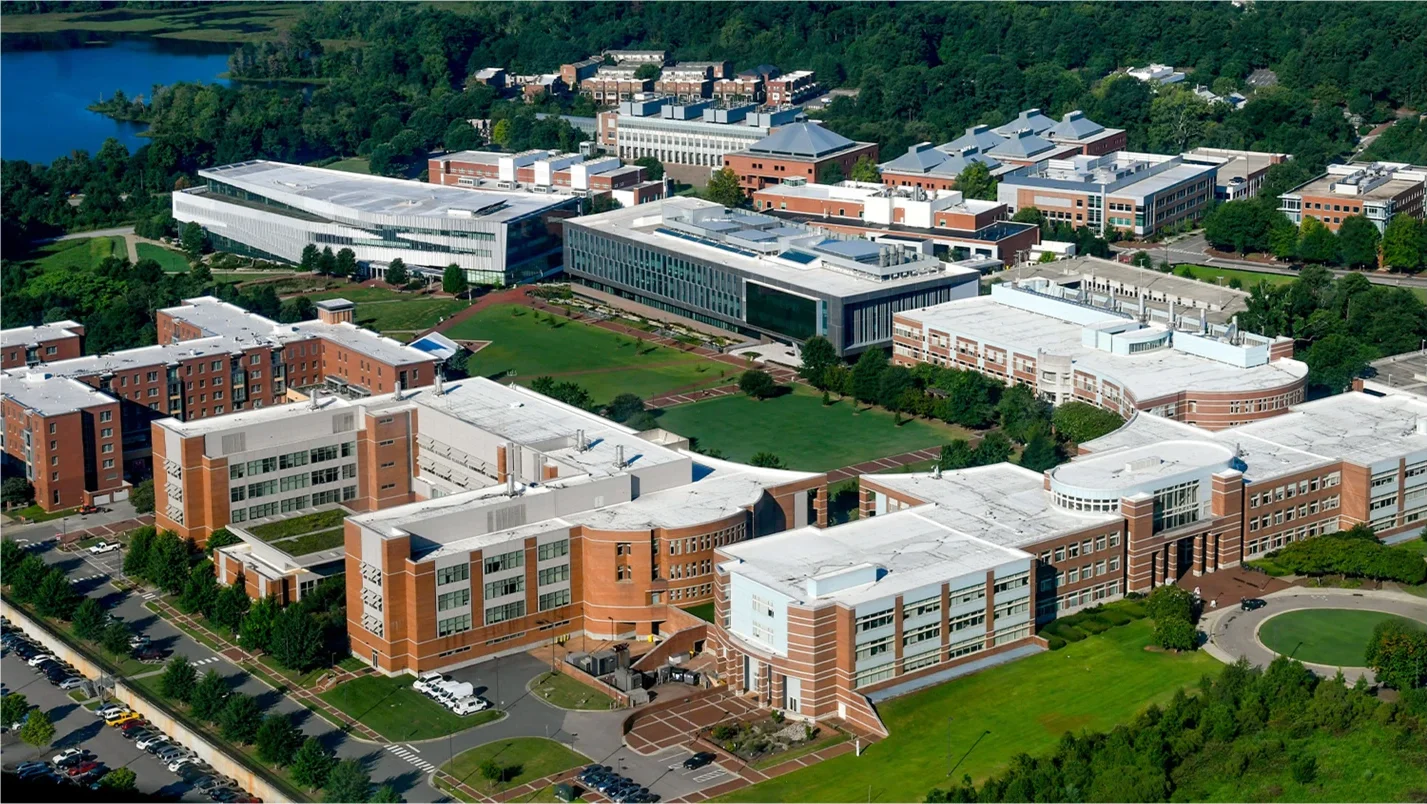
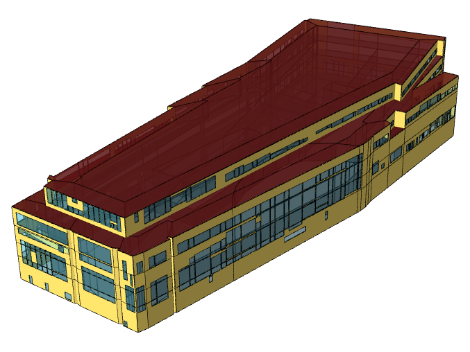
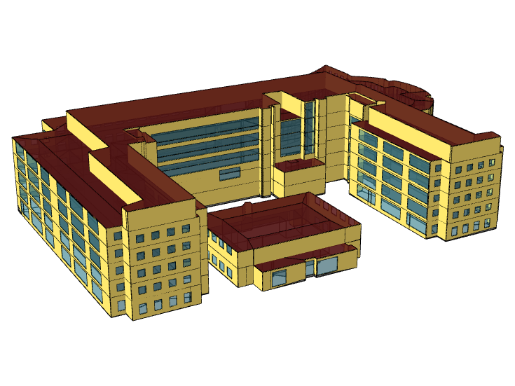
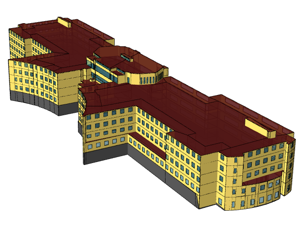
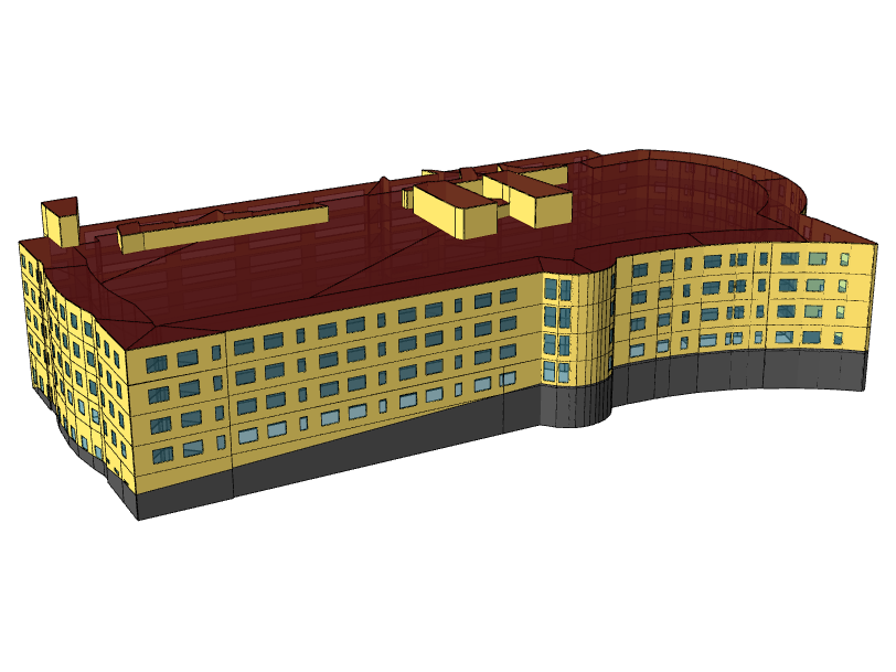
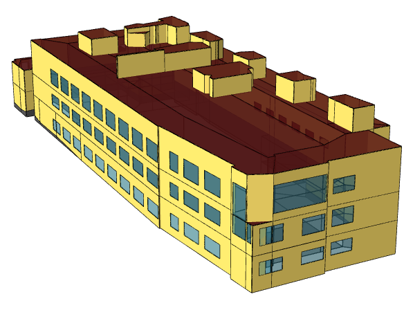
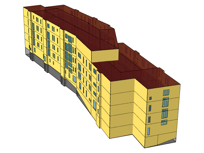
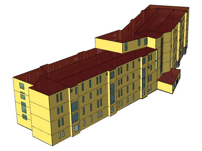
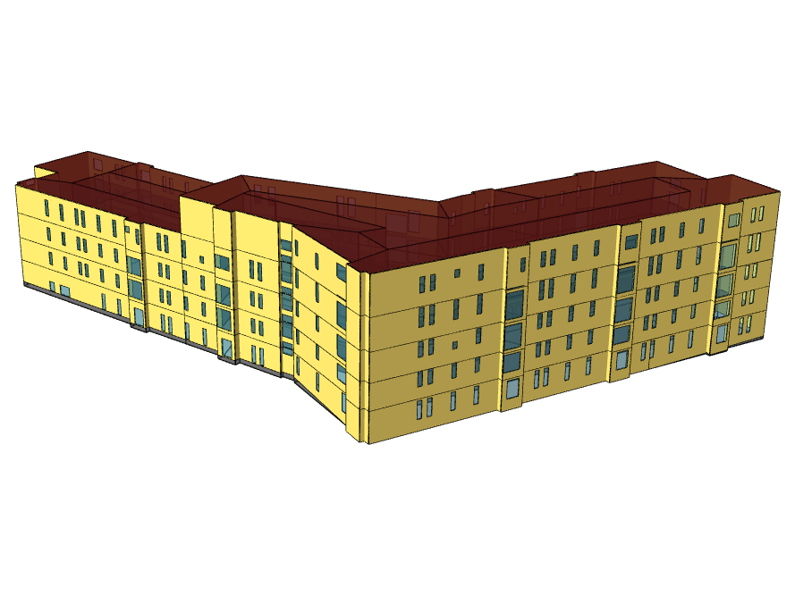
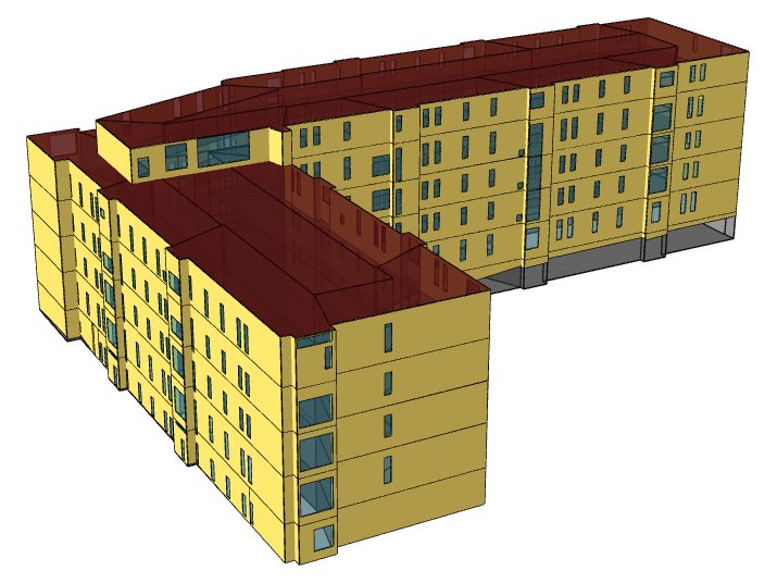
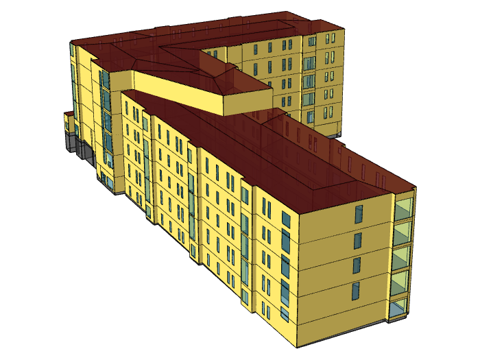
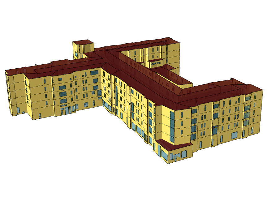
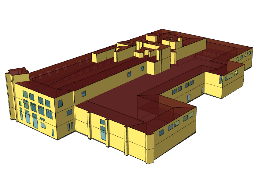
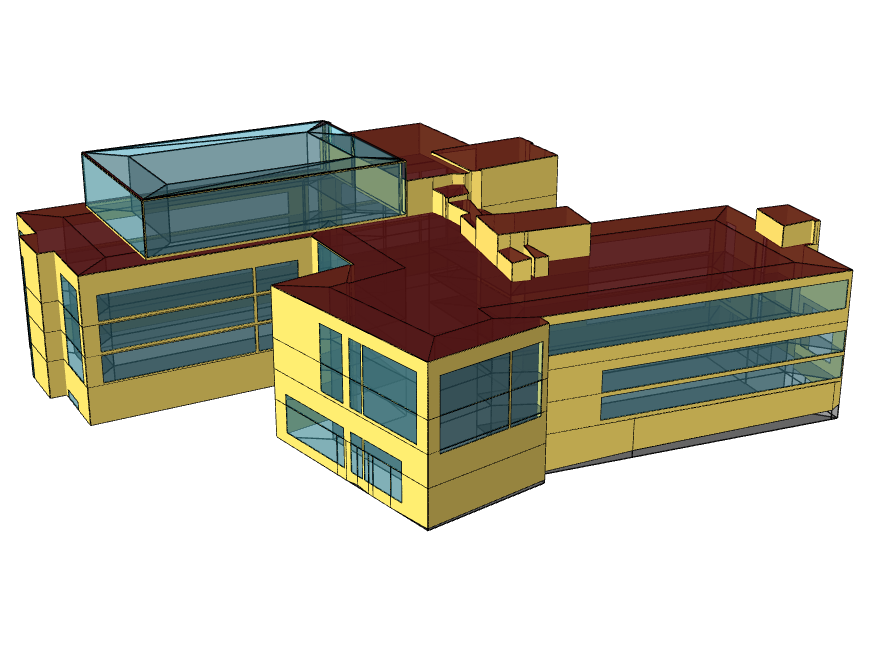
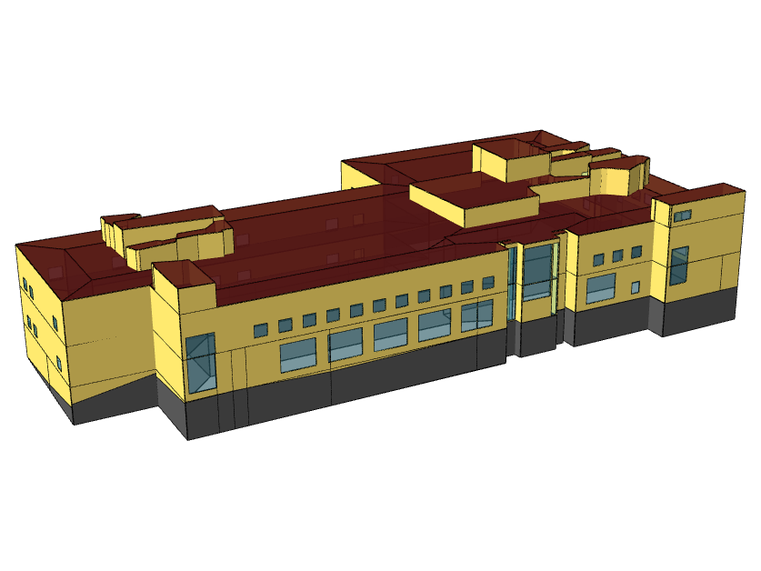
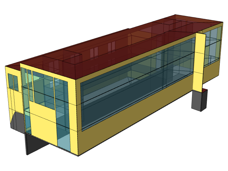
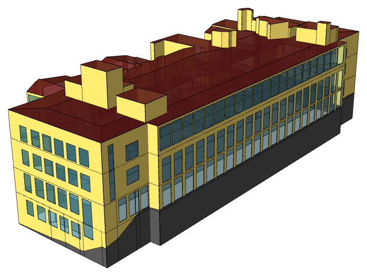
This work develops building energy models for the 20 buildings on NC State University’s Centennial Campus that are served by the district cooling system of the Centennial Campus Utility Plant (CCUP). Together with a model of the CCUP district cooling plant, the building models represent the campus district cooling system from the central plant to each connected building.
Building Energy Modeling
The 20 buildings connected to the CCUP district cooling system were built between 1990 and 2022 and include offices, laboratories, classrooms, a library, and residence halls, with a combined gross floor area of about 2.71 million ft² (about 252,000 m²) (Table 1).
Table 1. Buildings connected to the CCUP district cooling system
| No. | Building | Bldg. No. | Abbr. | Use | Year built | Floors | Gross floor area (ft²) |
|---|---|---|---|---|---|---|---|
| 1 | Center for Technology and Innovation | 702 | CTI | Office | 2016 | 3 | 71,726 |
| 2 | Constructed Facilities Laboratory | 720C | ERC | Laboratory | 1997 | 3 | 25,357 |
| 3 | Monteith Engineering Research Center | 720A | MRC | Office | 1997 | 5 | 121,623 |
| 4 | Poulton Innovation Center | 781A | PIC | Office | 1991 | 5 | 79,403 |
| 5 | Textiles Complex | 700 | TEX | Mixed-use complex | 1990 | 7 | 304,230 |
| 6 | Golden LEAF Biomanufacturing Training and Education Center (BTEC) | 762A | BTC | Office | 2007 | 4 | 87,897 |
| 7 | Plant Sciences Building | 763 | PSB | Classroom / Office / Laboratory | 2022 | 5 | 187,839 |
| 8 | Partners Building I | 775 | PT1 | Office | 1997 | 3 | 85,919 |
| 9 | Partners Building III | 713 | PT3 | Office | 2004 | 4 | 82,987 |
| 10 | Engineering Building I | 782A | EB1 | Classroom / Office | 2004 | 5 | 159,832 |
| 11 | Engineering Building II | 782B | EB2 | Classroom / Office | 2005 | 5 | 228,296 |
| 12 | Engineering Building III | 782C | EB3 | Classroom / Office | 2010 | 5 | 252,042 |
| 13 | James B. Hunt Jr. Centennial Campus Library | 783A | JHL | Library | 2012 | 6 | 243,559 |
| 14 | Fitts-Woolard Hall | 782E | FWH | Classroom / Office | 2020 | 5 | 229,893 |
| 15 | Tower Hall (Wolf Ridge Building 1) | 780A | WR1 | Residence hall / Restaurant | 2013 | 5 | 151,127 |
| 16 | Plaza Hall (Wolf Ridge Building 2) | 780B | WR2 | Residence hall | 2013 | 6 | 95,471 |
| 17 | Albright Innovation Hall (Wolf Ridge Building 3) | 780C | WR3 | Residence hall | 2014 | 6 | 90,841 |
| 18 | Valley Hall (Wolf Ridge Building 4) | 780D | WR4 | Residence hall | 2014 | 5 | 84,458 |
| 19 | Grove Hall (Wolf Ridge Building 5) | 780E | WR5 | Residence hall | 2014 | 5 | 62,358 |
| 20 | Lakeview Hall (Wolf Ridge Building 6) | 780F | WR6 | Residence hall | 2013 | 6 | 67,015 |
| Total | 2,711,873 | ||||||
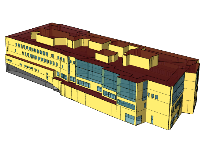
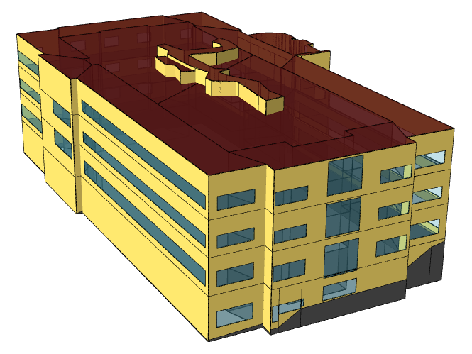
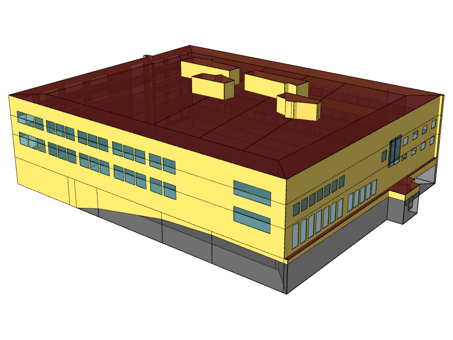
Each building is modeled individually, including its geometry and the window and curtain-wall openings on each facade (Figure 2). An interactive 3D view of the same buildings is available under GIS Modeling · LOD 3 Level.
Model Calibration
Both the district cooling plant model and the building models are calibrated against measured data. Calibration of the plant model is complete, and calibration of the 20 building models is in progress (Table 2).
Table 2. Calibration status of the plant and building models
| Model | Measured data | Status |
|---|---|---|
| CCUP district cooling plant | Plant operating data | Calibrated |
| 20 building energy models | Hourly data from each building | Calibration in progress |
Each building model is compared with its own building’s measured data at an hourly time step, following ASHRAE Guideline 14, using three statistical indicators:
- CV(RMSE) (coefficient of variation of the root mean square error): how widely the hourly predictions scatter around the measurements. Guideline 14 accepts hourly calibration at 30% or less.
- NMBE (normalized mean bias error): whether the model systematically over- or under-predicts. Guideline 14 accepts hourly calibration within ±10%.
- R² (coefficient of determination): how closely the simulated hourly profile follows the measured one.
NC State Campus Building and District System Modeling
Combined Heat and Power (CHP) Plant
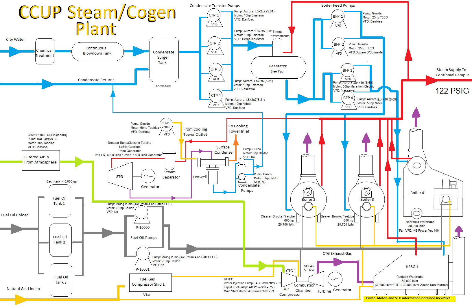
The Centennial Campus Central Utility Plant (CCUP) supplies steam to Centennial Campus at 122 psig through a combined heat and power (CHP) system. A 5.5 MW combustion turbine generator exhausts into a heat-recovery steam generator (HRSG) with a duct burner, and a 954 kW steam turbine generator, three boilers, and the condensate and boiler-feed systems complete the plant; the fuel supply is natural gas and fuel oil.
GIS Modeling
Overview
This work develops city-scale 3D building models of Raleigh, North Carolina and the NC STATE University Campus, organized by the Level of Detail (LoD) concept of the OGC CityGML 3.0 standard, with attributes for every building (use, height, year built, heating fuel). Building on these models and Urban Building Energy Modeling (UBEM), future research aims to develop a city-scale decarbonization model that evaluates retrofit and electrification scenarios and coordinates efficiency, flexibility and control under distribution grid constraints. The framework is designed to scale from campus and district level to entire cities across diverse urban conditions.
| Level | What is modelled | Main data | Area |
|---|---|---|---|
| LOD 1 | Block model: each footprint extruded to a single roof height (flat roof) | Building footprints + LiDAR roof heights | City of Raleigh · 156,326 buildings |
| LOD 2 | Adds the roof shape: roof planes fitted to the LiDAR point cloud | 2024 QL1 airborne LiDAR (high density, ≥ 8 points/m²) | Downtown Raleigh · 920 buildings |
| LOD 3 | Adds facade detail: windows, curtain walls, doors and rooftop PV as their own objects, with window-to-wall ratio per facade | Building drawings, Street View | Centennial Campus · 20 CCUP-connected buildings |
Future Land Use and Representative Districts
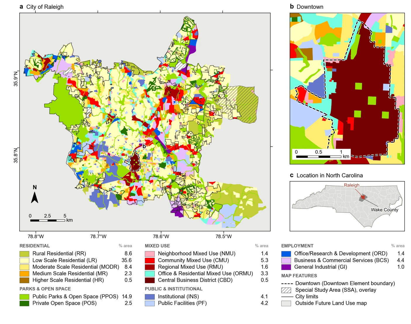
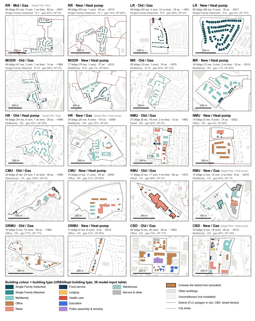
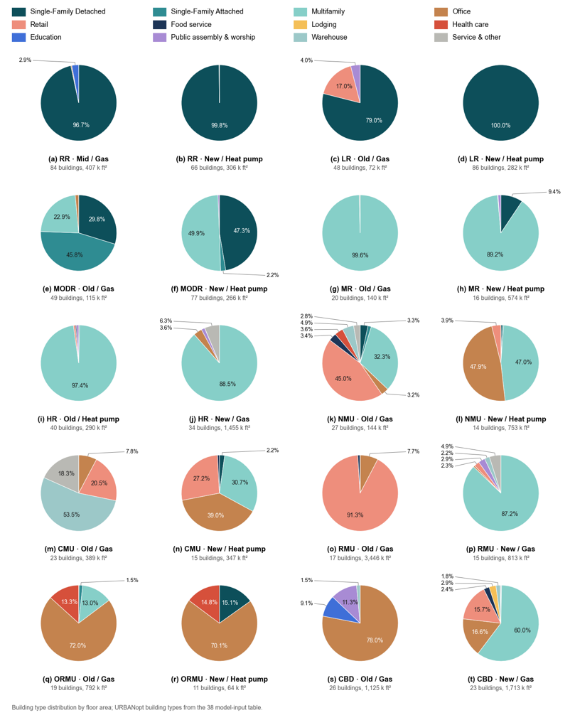
To carry the building models to district scale, 20 representative districts are selected from the City of Raleigh’s Future Land Use (FLU) map: for each of the ten FLU categories, one older, gas-heated district and one newer, heat-pump-heated district (Figures 1 and 2). Figure 3 shows the building-type mix of each district by floor area.
GIS Modeling · LOD 1 Level
City of Raleigh
Raleigh City 3D · LoD1 Blocks
Every building in the City of Raleigh (156,326 footprints) extruded to its roof height from the 2024 QL1 airborne LiDAR as an LoD1 block model. Use the panel on the left of the viewer to colour the buildings by type, land use, floors, year or heating fuel, add roads, sidewalks, lakes, green space, electric lines and substations, or jump to a place; hover a building for its details.
· Open in a new tab ↗ · drag to pan, right-drag to tilt, scroll to zoom, hover a building.
GIS Modeling · LOD 2 Level
City of Raleigh (Downtown)
Raleigh Downtown 3D · LoD2 Roofs
The 920 buildings in and around Raleigh's Central Business District with roof shapes reconstructed from the 2024 QL1 airborne LiDAR (LoD2). Switch between LoD1 blocks and LoD2 roofs, colour the buildings by use, year built or heating, and point at a building for its details.
· Open in a new tab ↗ · drag to orbit, scroll to zoom, right-drag to pan, point at a building.
GIS Modeling · LOD 3 Level
NC STATE Campus (Centennial Campus)
Centennial Campus 3D · LoD3 Buildings
The 20 Centennial Campus buildings on the Central Utility Plant (CCUP) chilled-water loop at Level of Detail 3, modelled from building drawings and Street View: walls, roofs, window and curtain-wall openings, doors and rooftop PV, with window counts and window-to-wall ratios (WWR) by facade. The rest of the campus is shown at LoD2 (LiDAR roof shapes). Pick a building to see its facade breakdown and jump to its east, west, north or south side; hover a building for its details.
· Open in a new tab ↗ · drag to pan, right-drag to tilt, scroll to zoom, hover a building.